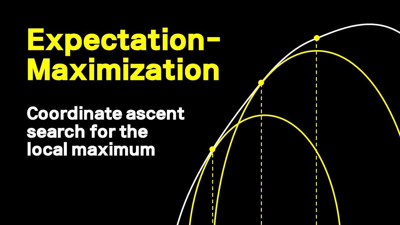
For an observed data $\mathbf{x}$, we might posit the existence of an unobserved data $\mathbf{z}$ and include it in model $p(\mathbf{x,z}\mid \theta)$. This is called a latent variable model. The question is, why bother? It turns out that in many cases, learning $\theta$ with the marginal log likelihood $p(\mathbf{x}\mid \theta)$ is hard, whereas learning with the joint likelihood with a complete data set $p(\mathbf{x,z}\mid \theta)$ is relatively easy. GMM is one such case.

Mixtures of Gaussians (GMM) GMM as a joint distribution Suppose a random vector $\mathbf{x}$ follows a $K$ Gaussian mixture distribution, $$ p(\mathbf{x}) = \sum_{k=1}^K \pi_k N(\mathbf{x}\mid \boldsymbol{\mu_k, \Sigma_k}) $$ Knowing the distribution means we have complete information about the set of parameters $\pi_k, \boldsymbol{\mu_k, \Sigma_k}$ for all $k$. Let us say that the parameter $\pi_k$ is shrouded, and instead we have a random variable $\mathbf{z}$ with $1-to-K$ coding where exactly one of $K$ elements (say $z_k$) be $1$ while all else are $0$.

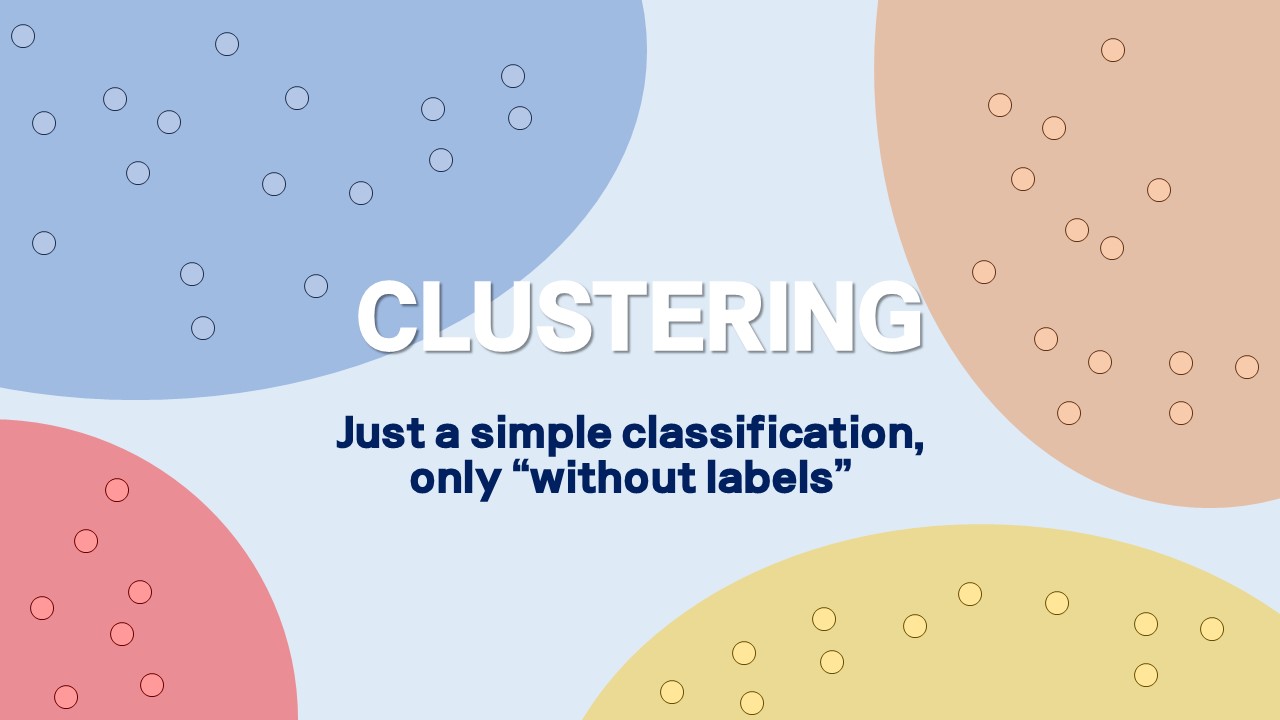
Gaussian mixture model is a widely used probabilistic model. For inference (model learning), we may use either EM algorithm which is a MLE approach or use Bayesian approach, which leads to variational inference. We would study this topic next week. For now, let us introduce one of the well-known nonparameteric methods for unsupervised learning, and introduce Gaussian mixture as a parametric counterpart. K-means clustering Let us suppose that we know the total number of clusters is fixed as $K$.

Review: Full conditional posterior for normal likelihood 일단 정규분포의 semi-conjugate prior에 대한 내용을 다시 정리해보자. $p(\theta\mid\sigma^2, \mathbf{D}) = dnorm(\theta, \mu_n, \tau_n^2)$ $\mu_n= \dfrac{1/\tau_0^2}{\frac{1}{\tau_0^2} + \frac{n}{\sigma^2}}\mu_0 + \dfrac{\frac{n}{\sigma^2}}{\frac{1}{\tau_0^2} + \frac{n}{\sigma^2}}\bar{x}$ $\tau_n^2 = \dfrac{1}{\frac{1}{\tau_0^2} + \frac{n}{\sigma^2}}$ $p(\sigma^2\mid\theta, \mathbf{D}) = dinv\Gamma(\sigma^2, v_n, \dfrac{1}{v_n}(v_0\sigma_0^2+\sum (y_i-\theta)^2)$ Two Group Comparison: Math scores library(ggplot2) library(cowplot) school1 = dget('http://www2.stat.duke.edu/~pdh10/FCBS/Inline/y.school1') school2 = dget('http://www2.stat.duke.edu/~pdh10/FCBS/Inline/y.school2') df = data.frame(school = c(rep('s1', length(school1)),rep('s2', length(school2))), score = c(school1, school2) ) ggplot(df, aes(x=school, y=score))+ geom_boxplot(aes(fill=school))+ ggtitle('Math scores comparison')+ theme_cowplot() 통계학이 필요한 이유는 이런 “애매한” 차이 때문이다.

0. 개요 베이지안에서 모수에 대한 추론은 곧 모수의 분포를 구하는 것이다. 미지의 수에 대한 불확실성을 확률로 표현하였으니, 베이즈 정리를 이용해 데이터의 불확실성과 거짓말처럼 깔끔하게 같이 섞을 수 있기 때문이다. 그러나 아쉽게도 그 결과로 나오는 분포는 항상 깔끔하지만은 않다. 물론 데이터에 대한 모델을 지수분포족으로 한정하고, 그에 대응하는 또다른 특별한 지수분포족 분포함수를 사용하면, 사후분포의 모수를 쉽게 구할 수 있는데, 이러한 경우를 Prior-Posterior 간에 Conjugacy가 있다고 한다. 그러나 많은 경우 복잡한 데이터에 맞게 모델을 만들다 보면 해석적이지 않은 사후분포에 맞닥뜨리게 된다.

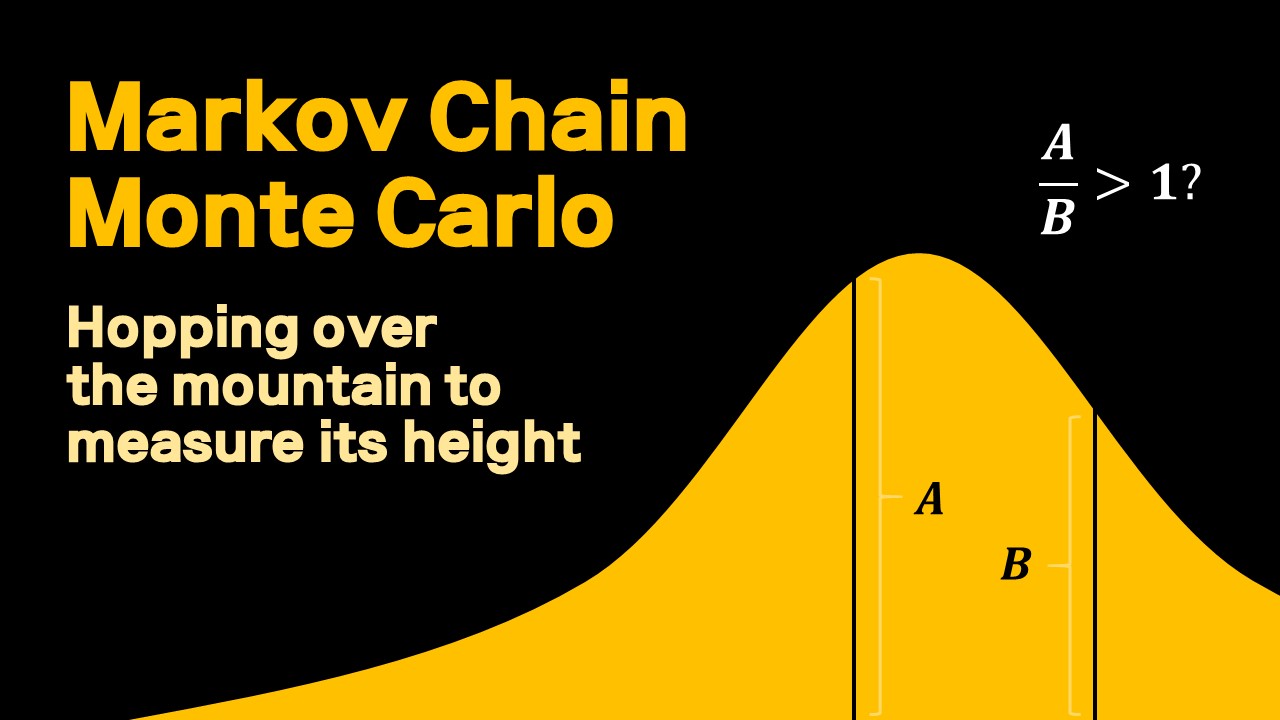
0. 이걸 왜 배우는데? 저번 시간에 간략히 살펴본 Gibbs Sampler는 MCMC(Markov Chain Monte Carlo), 즉 마코브 체인을 이용한 Posterior 분포 시뮬레이션 방법 중 하나인데, 이 MCMC 방법들이 도대체가 왜 잘 먹히는 지를 알려면 아무래도 마코브 체인에 대한 배경지식이 필요하다. 어떤 분포를 MCMC로 근사한다는 것은 모수 공간의 어떤 포인트에서 다른 포인트로 총총 점프하는 그 과정을 “잘” 구현해서, 마치 그 샘플들이 내가 모르는 그 분포에서 나온 것과 같다고 퉁치는 거다. MCMC 이름의 의미

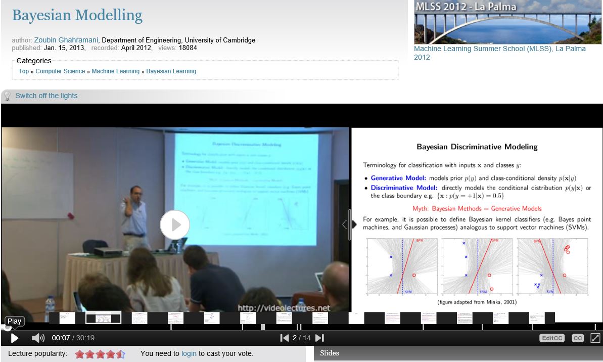
베이지안 머신러닝에 대해 인터넷에서 자료를 찾다보니 꽤 괜찮은 동영상 강의가 있어서 요약해보았다. 베이지안 모델링에 대해 개괄적으로 설명해주는 강의인데, 머신러닝에서 베이즈 정리가 어떻게 쓰이는지 잘 설명된 자료인 것 같다. http://videolectures.net/mlss2012_ghahramani_bayesian_modelling/ 위 링크에서 해당 강의 자료를 다운받고 시청할 수 있다. 다만 어도비 플래시가 있어야 구동이 되니 아마 올해가 지나면 못 듣지 않을까 싶다. 베이지안 모델링 외에도 Bayesian Nonparametrics, Graphical Model 등등 다른 다양한 강의가 있으니 한번 참고해보자. 아래에다가 강의 슬라이드별로 강의에서 아저씨가 말씀하신 부분을 나름 보충을 섞어 요약해놨다.