library(ggplot2) library(cowplot) library(reshape) Multivariate Normal Model Consider a bivariate normal random variable $[y_1, y_2]^T$. The density is written as ($p=2$)
$$ p(\mathbf{y}|\theta, \Sigma) = (\dfrac{1}{2\pi})^{-p/2}|\Sigma|^{-1/2} \exp{-\dfrac{1}{2}(\mathbf{y}-\theta)^T\Sigma^{-1}(\mathbf{y}-\theta)} $$
where the parameter is $\theta = \begin{pmatrix} E[y_1]\\\ E[y_2] \end{pmatrix}$ and $\Sigma = \begin{pmatrix} E[y_1^2]-E[y_1]^2 & E[y_1y_2]-E[y_1]E[y_2]\\\
E[y_2y_1]-E[y_2]E[y_1] & E[y_2^2]-E[y_2]^2 \end{pmatrix}$ $=\begin{pmatrix} \sigma_1^2 & \sigma_{12}\\\
\sigma_{21} & \sigma_2^1 \end{pmatrix}$.
Few things worth mentioning for multivariate normal model
the term in the exponent $(\mathbf{y}-\theta)^T\Sigma^{-1}(\mathbf{y}-\theta)$ is somewhat a measure of distance between mean and the data.
Inference for Normal Model Normal likelihood model has two parameters
$$ p(x|\theta, \sigma^2) = \dfrac{1}{\sigma\sqrt{2\pi}}\exp(-\dfrac{1}{2}(\dfrac{x-\theta}{\sigma})^2) $$ which requires a joint prior $p(\theta, \sigma^2)$. As for a single parameter case, we have joint posterior updated as
$$ p(\theta, \sigma^2|\mathbf{D}) \propto p(\theta, \sigma^2)p(\mathbf{D}|\theta, \sigma^2) $$ When our interest is in $\theta$, $\sigma^2$ is a nuisance parameter. Given the data $\mathbf{D}$ and the normal likelihood, we have three ways to deal with $\sigma^2$;
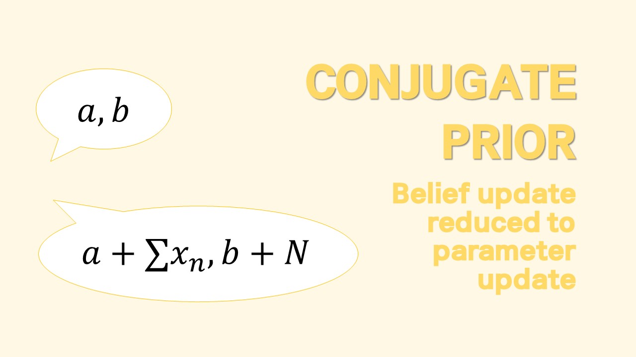
library(ggplot2) library(cowplot) library(reshape) Bayesian Update and Prediction Given a data $\mathbf{D}={x_1, x_2, …, x_n}$, once a likelihood model $p(\mathbf{D}|\theta)$ and a prior on a parameter $p(\theta)$ are specified, Bayesian inference produces an updated belief on $\theta$.
$$ \begin{align} \text{Prior Belief}&\quad p(\theta)\\\
\text{Likelihood}&\quad p(\mathbf{D}|\theta)\\\
\text{Updated (Posterior)}&\quad p(\theta|\mathbf{D}) = \dfrac{p(\mathbf{D}|\theta)p(\theta)}{\int p(\mathbf{D}|\theta)p(\theta)d\theta} \propto p(\mathbf{D}|\theta)p(\theta) \end{align} $$
Our interest may extend to the prediction the new value $\tilde{x}$ that would be generated from the same sampling distribution.
0. 생각하는 로봇은 베이지안이다! 주변 환경을 인지하고 목적지를 찾는 로봇을 생각해보자. 목적지로 가는 경로에는 수많은 경우의 수가 있다. 이 경로에서 로봇은 시시각각 환경을 파악해서, 즉 데이터를 수집해서 가장 안전한 길을 택해야 한다. 전방에 위험징후를 포착했다. 로봇은 그 방향으로 가는 길이 위험하다고 판단해 경로를 변경해야 한다. 자 그러면 이걸 어떻게 코딩할까? 각각의 길이 위험할 확률 $p(road_i=unsafe)$과, 각각의 길에서 위험한 징후가 포착될 확률 $p(sign\mid road_i=unsafe)$ 을 고려하여, 위험할 확률 $p(road_i = unsafe \mid sign)$ 을 다시 계산해야한다.
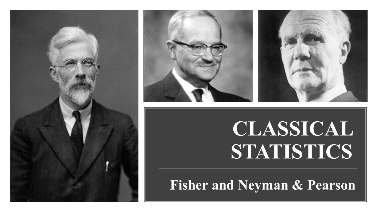
1. 빈도론적 추론의 병폐 자 이제 빈도통계론의 논리도 이해했고 그 끝판왕인 MLE와 LRT도 봤습니다. 지금부터는 빈도론적 통계 추론, 그 중에서도 검정 (NHST)이 가진 “병폐"들에 대해서 살펴보겠습니다. 앞서 잠깐 봤는데, 여기서는 좀 더 자세하게 다뤄보겠습니다.
1) Trigger Happy: $p(D \mid H_0)$만 보고 $H_0$을 기각함 $p(D\mid H_0)$이 굉장히 작아야지만 귀무가설을 기각하는 것이 얼핏 보면 굉장히 보수적으로 보이지만, 사실 이런 식으로 세팅을 해놓으면 “귀무가설에 반대되는 evidence"만 반영하게 되지, 귀무가설에 좋은 evidence는 절대 반영을 못함.
지금까지의 논의를 종합해보면 다음과 같습니다.
빈도통계학 추론은 평행우주 데이터 ${D^{(s)}}_{s=1}^{\infty}$에서의 Sampling Distrubtion $\delta(D^{(s)}) \sim p(.\mid \theta^*)$에 달렸다.
모수 $\theta$에 대한 추정량 $\hat{\theta} = \delta(D^{(s)})$의 결정은 다음의 사항을 고려해야 한다.
일단 $\delta$의 sampling distribtion을 근사적으로나마 알아야 한다.
가급적이면 $\delta$의 평행우주 데이터 ${D^{(s)}}_{s=1}^{\infty}$에서의 행태가 “이쁘면” 좋겠다. (Consistent, Unbiased, Efficient)
Sampling distribution $\delta(D^{(s)}) \sim p(.\mid\theta^*)$만 알면 점 추정, 구간 추정, 가설 검정 다 할 수 있다!
빈도론자들의 세계관을 다시 한번 복기해봅시다. 데이터의 sampling density를 모수 $\theta$로 결정되는 확률분포함수로 가정하였고, $\theta$를 모를 때 이 sampling density를 데이터에 의해 정해지는 $\theta$의 식인 Likelihood로 해석합니다. 비록 우리가 가진 샘플은 $D^{(s)}$ 하나이지만 내가 모르는 수많은 평행우주에 똑같은 확률실험의 결과들의 앙상블인 ${D^{(s)}}_{s=1}^{\infty}$가 있다고 믿어봅시다.
$$ \begin{align} \text{Ensemble of Data:}\quad & D_{s=1}^{\infty} = [x_1^{(s)}, x_2^{(s)}, …, x_n^{(s)}]_{s=1}^{\infty}\\\
\text{Sampling Density of $D^{(s)}$ (iid):}\quad& f(D^{(s)}|\theta) = \prod_{i=1}^nf(x_i^{(s)}|\theta) \quad (x_i^{(s)}\in \mathcal{X}, \theta \in \Omega)\\\
\text{Likelihood of $\theta$ given $D^{(s)}$:}\quad& L(\theta|D^{(s)}) \end{align} $$ 우리는 데이터를 보고 모수를 추정하고자 합니다.