library(ggplot2)
library(cowplot)
library(reshape)

Bayesian Update and Prediction

Given a data $\mathbf{D}={x_1, x_2, …, x_n}$, once a likelihood model $p(\mathbf{D}|\theta)$ and a prior on a parameter $p(\theta)$ are specified, Bayesian inference produces an updated belief on $\theta$.

$$ \begin{align} \text{Prior Belief}&\quad p(\theta)\\\
\text{Likelihood}&\quad p(\mathbf{D}|\theta)\\\
\text{Updated (Posterior)}&\quad p(\theta|\mathbf{D}) = \dfrac{p(\mathbf{D}|\theta)p(\theta)}{\int p(\mathbf{D}|\theta)p(\theta)d\theta} \propto p(\mathbf{D}|\theta)p(\theta) \end{align} $$

Our interest may extend to the prediction the new value $\tilde{x}$ that would be generated from the same sampling distribution. This is obtanind by taking a weighted average of $p(\tilde{x}|\theta)$ over all the possible $\theta$. $p(\tilde{x})$ is called a prior predictive distribution where the weight is the belief prior to the data. $p(\tilde{x}|\mathbf{D})$ is called posterior predictive distribution as its weight is updated per data.

$$ \begin{align} \text{Prior predictive}&\quad p(\tilde{x}) = \int p(\tilde{x}|\theta)p(\theta)d\theta\\\
\text{Posterior predictive}&\quad p(\tilde{x}|\mathbf{D}) = \int p(\tilde{x}|\theta)p(\theta|\mathbf{D})d\theta \end{align} $$

Gamma-Poisson Model

Poisson likelihood is often used for modelling a distribution of counts.

$$ p(x|\theta) = \dfrac{\theta^x e^{-\theta}}{x!} \quad (x\in \mathcal{X}={0, 1, 2,…}) $$

For $\mathbf{D} = {x_1, x_2, …,x_n}$ we have joint likelihood

$$ \begin{align} \text{Poisson likelihood}\quad p(\mathbf{D}|\theta) &= \prod_{i=1}^n\dfrac{\theta^{x_i} e^{-\theta}}{x_i!} = c(x_1, x_2, …, x_n) \theta^{\sum_{i}x_i}e^{-n\theta} \end{align} $$

Give any prior $p(\theta)$, the posterior would be

$$ \begin{align} p(\theta|\mathbf{D}) \propto p(\theta, \mathbf{D}) &= p(\theta)p(\mathbf{D}|\theta)\\\
&= p(\theta) \theta^{\sum_{i}x_i}e^{-n\theta} \end{align} $$

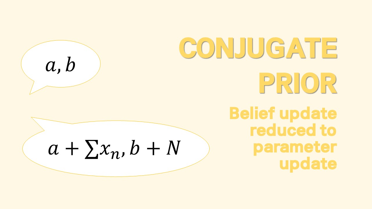
For $p(\theta)$ to be conjugate, i.e. for $p(\theta)$ to be in same form as $p(\theta|\mathbf{D})$, the prior must contain a term $\theta^{c_1}e^{-c_2}$. A natural choice for the prior would be gamma density $\theta \sim \Gamma(a,b)$

$$ \text{Gamma prior}\quad p(\theta) = \dfrac{b^a}{\Gamma(a)}\theta^{a-1}e^{-b\theta} $$

Then we can easily see that the posterior is given as $\theta|\mathbf{D} \sim \Gamma(a+\sum_{i}x_i, b+n)$

$$ \text{Gamma posterior}\quad p(\theta|\mathbf{D}) = \dfrac{(b+n)^{(a+\sum x_i)}}{\Gamma(a+\sum x_i)}\theta^{a+\sum x_i-1}e^{-\theta(b+n)} $$

with mean and variance

$$ \begin{align} E[\theta] &= \dfrac{a+\sum_{i}x_i}{b+n} = \dfrac{b}{b+n}\dfrac{a}{b} + \dfrac{n}{b+n}\dfrac{\sum_ix_i}{n}\
V[\theta] &= \dfrac{a+\sum_{i}x_i}{(b+n)^2} \end{align} $$

Two points worth noted;

• The prior parameter $a$ means “prior sample counts”, and $b$ means “prior sample size”. ($a$ counts among $b$ samples)

• As $n\to \infty$, $E[\theta] \to \bar{x}$ and $V[\theta] \to \bar{x}/n$. We can see that for large $n$, the prior information is dominated by the sample likelihood.

Posterior predictive distribtion for prediction of new value $\tilde{x}$ can be obtained from

$$ \begin{align} p(x|\mathbf{D})&= \int p(x|\theta)p(\theta|\mathbf{D})d\theta\\\
&= \int \dfrac{\theta^x e^{-\theta}}{x!}\dfrac{(b+n)^{(a+\sum x_i)}} {\Gamma(a+\sum x_i)}\theta^{a+\sum x_i-1}e^{-\theta(b+n)} d\theta\\\
&= \dfrac{(b+n)^{(a+\sum x_i)}}{\Gamma(x+1)\Gamma(a+\sum x_i)} \int \theta^{a+\sum x_i + x -1} e^{-(b+n+1)\theta}d\theta\\\
&= \dfrac{\Gamma(a+\sum x_i+x)}{\Gamma(x+1)\Gamma(a+\sum x_i)} (\dfrac{b+n}{b+n+1})^{a+\sum x_i}(\dfrac{1}{b+n+1})^{x}\\\
&= {x+a+\sum x_i -1 \choose a+\sum x_i -1} (\dfrac{b+n}{b+n+1})^{a+\sum x_i}(\dfrac{1}{b+n+1})^{x} \end{align} $$

From this we can see that the posterior predictive distribution of Gamma-Poisson model is actually a negative binomial model with mean and variance

$$ \begin{align} \text{Posterior predictive}\quad & x|\mathbf{D} \sim NB(a+\sum x_i, \dfrac{b+n}{b+n+1})\\\
\text{Posterior predictive mean}\quad & E[x|\mathbf{D}] = \dfrac{a+\sum x_i}{b+n} = E[\theta|\mathbf{D}]\\\
\text{Posterior predictive variance}\quad & V[x|\mathbf{D}] = \dfrac{a+\sum x_i}{b+n} \dfrac{b+n+1}{b+n} \\\
&= V[\theta|\mathbf{D}] ;(b+n+1)\\\
&= E[\theta|\mathbf{D}];(1+\dfrac{1}{b+n}) \end{align} $$

Compare this with the frequentist approach. In frequentist prediction for poisson model, we would obtain a single estimator say, mle, $\hat{\theta}$ for $\theta$, and this yields a predictive distribution $p(x|\hat{\theta})$ with $E[x|\hat{\theta}]=V[x|\hat{\theta}]=\hat{\theta}$. In Bayesian, since inference on the parameter is given as a distribution, not a single number, we have to marginalize out $\theta$. The marginalization leads to, rather incidentally, the negative binomial predictive distribution, and we have mean $E[\theta |\mathbf{D}]$ instead of $\hat{\theta}$, and variance $E[\theta|\mathbf{D}] (1+1/(b+n))$ instead of $\hat{\theta}$.

Posterior predictive variance implies an uncertainty about the new value of $x$. This uncertainty stems from

1. $E[\theta|\mathbf{D}]$: sampling variability inherent in the poisson likelihood model
2. $1+1/(b+n)$: mainly due to uncertainty in the true value of $\theta$.

Hence we can see that as $n \to \infty$, we have plenty of data for $\theta$ and the predictive variance reduces to $E[\theta|\mathbf{D}]$.

In summary,

$$ \begin{align} \text{Data} &\quad \mathbf{D} ={x_1, x_2, …, x_n}\\\
\text{Likelihood} &\quad x_i \sim poi(\theta)\\\
\\\
\text{Prior} &\quad \theta \sim \Gamma(a,b)\\\
\text{Posterior} &\quad \theta|\mathbf{D} \sim \Gamma(a+\sum x_i,b+n)\\\
\\\
\text{Posterior predictive} &\quad x|\mathbf{D} \sim NB(a+\sum x_i, \dfrac{b+n}{b+n+1})\\\
&E[x|\mathbf{D}] = E[\theta|\mathbf{D}]\\\
&V[x|\mathbf{D}]=E[\theta|\mathbf{D}];(1+\dfrac{1}{b+n}) \end{align} $$

Example: Birth Rates (FCBSM Ex 4.8)

Let $\theta_A$ and $\theta_B$ be the average number of children of men in their 30s with and without bachelor’s degrees, respectively. Accordingly, let $Y_{i,A}$, $Y_{i,B}$ be a number of child such that

$$ Y_{i,A} \sim poi(\theta_A)\\\
Y_{i,B} \sim poi(\theta_B) $$

and are given data where $n_A = 58, n_B = 305$ and $\sum Y_{i,A}=54, \sum Y_{i,B}=305$.

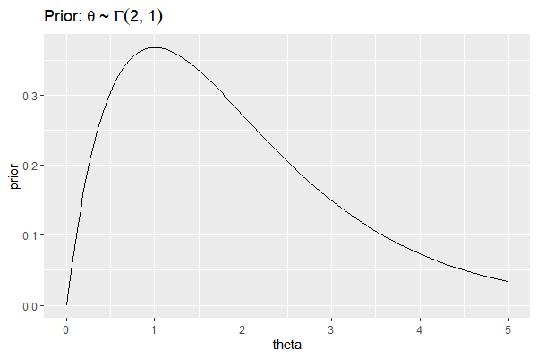
Suppose we have a prior belief in $\theta_A, \theta_B$ as follows

$$ \theta_A \sim \Gamma(2,1)\\\
\theta_B \sim \Gamma(2,1) $$

which can be plotted as

df=data.frame(
  theta = seq(0, 5, by=0.01),
  prior = dgamma(seq(0, 5, by=0.01), 2,1)
)
ggplot(df, aes(x=theta, y=prior))+
  geom_line()+
  ggtitle(bquote("Prior:"~theta~"~"~Gamma(2,1)))

menchild30bach=scan(url('http://www2.stat.duke.edu/~pdh10/FCBS/Exercises/menchild30bach.dat'))
menchild30nobach=scan(url('http://www2.stat.duke.edu/~pdh10/FCBS/Exercises/menchild30nobach.dat'))
c(sum(menchild30bach), length(menchild30bach))
c(sum(menchild30nobach), length(menchild30nobach))

# prior
a=2; b=1
theta= seq(0,5, by=0.01)
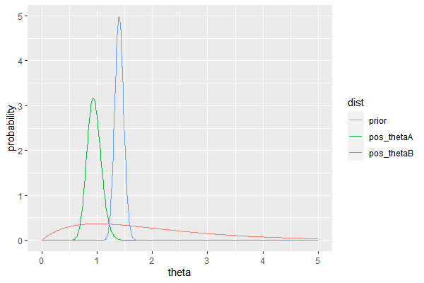
# posterior
df=data.frame(
  theta = theta,
  prior = dgamma(theta, a, b),
  pos_thetaA = dgamma(theta, a + sum(menchild30bach), b + length(menchild30bach)),
  pos_thetaB = dgamma(theta, a + sum(menchild30nobach), b + length(menchild30nobach))
)

df_long = melt(df, id.vars='theta', variable_name='dist')
ggplot(df_long, aes(x=theta, y=value, group=dist, color=dist))+
  geom_line()+
  ylab('probability')

We can sample from posterior predictive distribution as follows

# mc sample size
N=50000

# sample from posterior belief
thetaA = rgamma(N, a + sum(menchild30bach), b + length(menchild30bach))
thetaB = rgamma(N, a + sum(menchild30nobach), b + length(menchild30nobach))

# sample new values of Y
ynewA = rpois(N, thetaA)
ynewB = rpois(N, thetaB)

# Assemble
pos_predict = data.frame(
  ynew = c(ynewA, ynewB),
  dist = factor( rep(c('bach','nobach'), each=N), levels=c('bach','nobach')),
  type='posterior'
)

ggplot(pos_predict, aes(x=ynew, group=dist)) +
  geom_histogram() +
  facet_grid(.~dist)

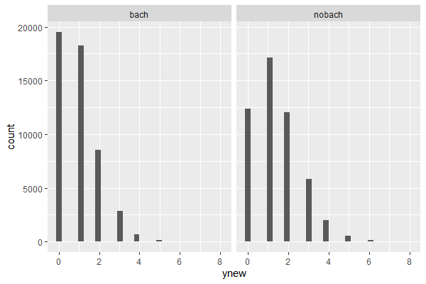
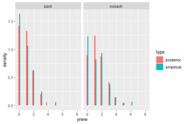
Compared with the empirical distribution, the model for “nobach” data poorly reflected counts for 0 and 1 child. This is not a big of a concern as long as the parameter in interest, which is in this case a mean of the distribution, is not significantly differenct from the data. However, if the very modelling purpose was to do an inference on a parameter such as a proportion of observations with 0 or 1 child, then our poisson model should be reconsidered, in favor of a more suitable model such as in this case a multinomial model. When modelling the distribution of the data. the primary criterion should be the parameters in question.

emp_df = data.frame(
  ynew = c(menchild30bach, menchild30nobach),
  dist = factor(c(rep('bach',length(menchild30bach)), rep('nobach',length(menchild30nobach))),
                levels=c('bach','nobach')),
  type='empirical'
)

total_df = rbind(pos_predict, emp_df)

ggplot(total_df, aes(x=ynew, y=..density.., group = type, fill=type))+
  geom_histogram(position='dodge')+
  facet_grid(. ~ dist)

d = 50 # number of factors (variables)
N = 2^17 # number of observation
p = runif(d) # different distribution for each factor

factor = function(p){return(rbinom(N, 1, p))}
output = sapply(p, factor) # generate distribution of factors
beta = runif(d)*2-1 # generate beta for each factor

df = data.frame(height = output %*% beta)

ggplot(df, aes(x=height)) + geom_histogram(color='black',fill='grey', bins=30)

References

1. First Course into Bayesian Statistical Analysis (Hoff, 2009)
2. https://github.com/jayelm/hoff-bayesian-statistics