
Conjugate Prior for Univariate - Normal Model
Inference for Normal Model
Normal likelihood model has two parameters
$$ p(x|\theta, \sigma^2) = \dfrac{1}{\sigma\sqrt{2\pi}}\exp(-\dfrac{1}{2}(\dfrac{x-\theta}{\sigma})^2) $$
which requires a joint prior $p(\theta, \sigma^2)$. As for a single parameter case, we have joint posterior updated as
$$ p(\theta, \sigma^2|\mathbf{D}) \propto p(\theta, \sigma^2)p(\mathbf{D}|\theta, \sigma^2) $$
When our interest is in $\theta$, $\sigma^2$ is a nuisance parameter. Given the data $\mathbf{D}$ and the normal likelihood, we have three ways to deal with $\sigma^2$;
- Assume $\sigma^2$ is known; $p(\theta, \sigma^2) = p(\theta|\sigma^2)$
- Give prior on $\theta$ conditional on $\sigma^2$, and give prior to $\sigma^2$ also; $p(\theta, \sigma^2)=p(\theta|\sigma^2)p(\sigma^2)$
- Give independent prior for both $\theta, \sigma^2$; $p(\theta, \sigma^2) = p(\theta)p(\sigma^2)$
The bottom line is, 1 and 2 still has conjuagte prior-posterior but deriving posterior for 3 is analytically impossible and requires numerical approximation.
Normal Model (known variance)
First note that the normal distribution takes the form
$$
\begin{align}
p(x|\theta, \sigma^2) &\propto \exp({-\frac{1}{2}(ax^2+bx+c)})\\\
\text{where}\quad &a = 1/\sigma^2 \rightarrow \sigma^2=1/a\\\
\text{and}\quad &b = -2\theta/\sigma^2 \rightarrow \theta = -b\sigma^2/2
\end{align}
$$
This skill is known as “completing the square”, and is useful in multiplying two distribtuion in form (38).
Now given the joint likelihood
$$ p(\mathbf{D}|\theta, \sigma^2) = (2\pi\sigma^2)^{-n/2}\exp(-\dfrac{1}{2}\sum(\dfrac{x_i-\theta}{\sigma})^2) $$
we have a posterior update for $\theta$ given as
$$
\begin{align}
p(\theta|\mathbf{D}, \sigma^2) &\propto p(\theta|\sigma^2)p(\mathbf{D}|\theta, \sigma^2)\\\
& \propto p(\theta|\sigma^2)\exp(c_1(\theta-c_2)^2)
\end{align}
$$
This means that the prior must contain a term similiar $\exp(c_1(\theta-c_2)^2)$, so the normal prior for $\theta$ becomes a natural choice. Let $\theta|\sigma^2 \sim N(\mu_0, \tau_0^2)$ and we have
$$
\begin{align}
p(\theta|\mathbf{D}, \sigma^2) &\propto p(\theta|\sigma^2)p(\mathbf{D}|\theta, \sigma^2)\\\
&\propto \exp(-\dfrac{1}{2\tau_0^2}(\theta - \mu_0)^2)\exp(-\dfrac{1}{2\sigma^2}\sum(\theta - x_i)^2)
\end{align}
$$
Since $\theta|\mathbf{D}, \sigma^2$ is also a normal distribution, we only need to figure out the posterior mean and variance. By expanding the exponential term in quadratic form and using the completing the square skill, we can see that
$$
\begin{align}
\theta|\sigma^2, \mathbf{D} & \sim N(\mu_n, \tau_n^2)\\\
\mu_n&= \dfrac{1/\tau_0^2}{1/\tau_0^2 + n/\sigma^2}\mu_0 + \dfrac{n/\sigma^2}{1/\tau_0^2 + n/\sigma^2}\bar{x}\\\
\tau_n^2 &= \dfrac{1}{1/\tau_0^2 + n/\sigma^2}
\end{align}
$$
In Bayesian context, an inverse of variance is often referred to as a precision. In this sense, $1/\tau_0^2$ is a precision of prior belief on $\mu_0$, and $n/\sigma^2$ is a precision on $\bar{x}$ based on the data.
For the sake of interpretability, we might set prior precision as $1/\tau_0^2 = \sigma^2/k_0$. In that case, the prior $\theta|\sigma^2 \sim N(\mu_0, \sigma^2/k_0)$ implies a belief that mean of the likelihood $\mathbf{D}|\theta,\sigma^2 \sim N(\theta, \sigma^2)$ is $\mu_0^2$ where $k_0$ essentially takes on a meaning of a prior sample size, and we have
$$
\begin{align}
\mu_n&= \dfrac{k_0}{k_0+n}\mu_0+\dfrac{n}{k_0+n}\bar{x}\\\
\tau_n^2 &= \dfrac{\sigma^2}{k_0+n}
\end{align}
$$
The posterior predictive $\tilde{x}|\mathbf{D}, \sigma^2$ is
$$ p(\tilde{x}|\mathbf{D}, \sigma^2) = \int p(\tilde{x}|\theta, \sigma^2)p(\theta|\mathbf{D}, \sigma^2) d\theta $$
Since the likelihood $\tilde{x}|\theta, \sigma^2$ and the posterior $\theta|\mathbf{D}, \sigma^2$ are both normal, its product which is in the integrand is a bivariate normal distribution, and therefore $p(\tilde{x}|\mathbf{D}, \sigma^2)$ is also normal. We can easily compute its mean and variance with a little trick and get full posterior predictive distribution as follows without having to solve the above integral.
$$
\begin{align}
E[\tilde{x}|\mathbf{D}, \sigma^2]&= E[E[\tilde{x}|\theta, \sigma^2, \mathbf{D}]|\sigma^2, \mathbf{D}] = E[\theta|\sigma^2, \mathbf{D}]=\mu_n\\\
V[\tilde{x}|\mathbf{D}, \sigma^2]&= E[V[\tilde{x}|\theta, \sigma^2, \mathbf{D}]|\sigma^2, \mathbf{D}] + V[E[\tilde{x}|\theta, \sigma^2, \mathbf{D}]|\sigma^2, \mathbf{D}]\\\
&= E[\sigma^2|\sigma^2, \mathbf{D}]+ V[\theta|\sigma^2, \mathbf{D}]\\\
&= \sigma^2 + \tau_n^2\\\
\therefore \tilde{x}|\mathbf{D},\sigma^2&\sim N(\mu_n, \sigma^2+\tau_n^2)
\end{align}
$$
A few points worth noted;
- The frequentist estimator for $\theta$ is $\bar{x}$, whereas the Bayesian estimator is $E[\theta|\sigma^2, \mathbf{D}] = w\mu_0 + (1-w)\bar{x}$. This is clearly a biased estimator, but since $\mu_0$ is a constant prior parameter and $1-w<1$, the variance is actually smaller then the frequentist estimator. Since $MSE=Bias^2+Variance$, if the bais induced by the prior mena $\mu_0$ is not so severe, than the Bayesian estimator for the population mean can acutally have less MSE than the sample mean.
- As in the Gamma-Poisson Model, the posterior predictive variance $V[\tilde{x}|\mathbf{D}, \sigma^2]$ consists of two parts; uncertainty in the center of the population $\tau_n^2$ and the sampling variability inherent in the normal likelihood $\sigma^2$. As $n \to \infty$, we get more certain on $\theta$ so $\tau_n^2\to 0$, and only left with $\sigma^2$.
Example: Midge wing length (known variance)
D = c(1.64, 1.70, 1.72, 1.74, 1.82, 1.82, 1.82, 1.90, 2.08)
mean(D)
var(D)
Our prior is $\theta \sim N(1.9, 0.95)$ based on previous research. Let $\sigma^2 = s^2$. Then the posterior of $\theta$ is normal with mean and variance
$$
\begin{align}
\mu_n &= \dfrac{1/0.95^2(1.9)+9/0.017(1.804)}{1/0.95^2 + 9/0.017}\\\
\tau_n^2 &= \dfrac{1}{1/0.95^2+9/0.017}
\end{align}
$$
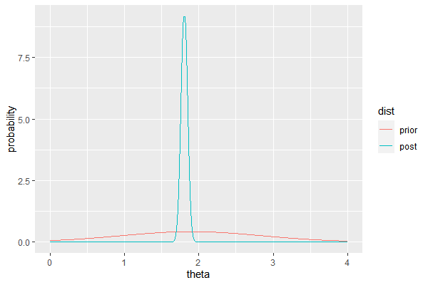
When plotted,
# prior
mu0=1.9; tau0=0.95

# data
N = length(D)
xbar = mean(D)
sigma = sd(D)

# posterior
mu1 = (mu0*1/tau0^2 + (length(D)/sigma^2)*xbar) / (1/tau0^2+length(D)/sigma^2)
tau1 = sqrt(1/(1/tau0^2+length(D)/sigma^2))

theta= seq(0,4, by=0.01)
df=data.frame(
  theta = theta,
  prior = dnorm(theta, mu0, tau0),
  post = dnorm(theta, mu1, tau1)
)

df_long = melt(df, id.vars='theta', variable_name='dist')
ggplot(df_long, aes(x=theta, y=value, group=dist, color=dist))+
  geom_line()+
  ylab('probability')
Normal Model (unknown variance, conditional prior)
Let us consider a prior where mean is conditional on the variance, as in the normal model with known variance, but there exists a prior for variance also. For the sake of simplicity let the prior on mean as $\theta|\sigma^2 \sim N(\mu_0, \sigma/\tau_0)$. Then we have
$$ p(\theta, \sigma^2) = dnorm(\theta|\mu_0, \sigma/\sqrt{k_0})p(\sigma^2) $$
We would seek a probaility density on $\sigma^2$ with a support on $\mathbb{R}_{+}$ and $\sigma^2|\mathbf{D}$ has $\sigma^2$ retains conjugacy. It turns out that the inverse gamma distribution for the variance $\sigma^2$ satisfies these requirements, which is equivalent to saying the precision has a gamma distribution.
Note: derivation of inverse-gamma density Let $x\sim \Gamma(a,b)$ with a density
$$ p(x) = \dfrac{b^a}{\Gamma(a)}x^{a-1}e^{-bx} $$
Let $y=1/x$ with $dx/dy = -1/y^2$ and we have
$$
\begin{align}
p(y) &= \dfrac{b^a}{\Gamma(a)}(\dfrac{1}{y})^{a-1}e^{-\frac{b}{y}}\mid\dfrac{1}{y^2}\mid\\\
&= \dfrac{b^a}{\Gamma(a)}(\dfrac{1}{y})^{a+1}e^{-\frac{b}{y}}
\end{align}
$$
For interpretability, let us consider a prior
$$
\begin{align}
\sigma^2 &\sim inv\Gamma(v_0/2, v_0\sigma^2_0/2)\\\
p(\sigma^2)&=\dfrac{(v_0\sigma^2_0/2)^{v_0/2}}{\Gamma(v_0/2)}(\dfrac{1}{\sigma^2})^{v_0/2+1}e^{-\frac{v_0\sigma^2_0/2}{\sigma^2}}
\end{align}
$$
In summary, we have
$$
\begin{align}
\sigma^2 &\sim inv\Gamma(v_0/2, v_0\sigma_0^2/2)\\\
\theta|\sigma^2 &\sim N(\mu_0, \sigma/k_0)\\\
\mathbf{D}|\theta, \sigma^2 &\sim N(\theta, \sigma^2)
\end{align}
$$
The conditional posterior for the mean $\theta|\sigma^2, \mathbf{D}$ is already given in (49), (50). The posterior for $\sigma^2$ requires some calculus.
$$
\begin{align}
p(\sigma^2|\mathbf{D})
&\propto p(\sigma^2) p(\mathbf{D}|\sigma^2)\\\
&= p(\sigma^2) \int p(\mathbf{D}|\theta,\sigma^2)p(\theta|\sigma^2) d\theta\\\
&=dinv\Gamma(\sigma^2, v_0/2, v_0\sigma_0^2/2)
\int \prod_{i} dnorm(x_i,\theta, \sigma^2)
dnorm(\theta, \mu_0, \sigma^2/k_0) d\theta\\\
&\propto (\dfrac{1}{\sigma^2})^{v_0/2+1}\exp(-\frac{v_0\sigma^2_0}{2\sigma^2})
(\dfrac{1}{\sigma^2})^{n/2}\exp(-\frac{1}{2}(\dfrac{\theta-\frac{k_0\mu_0+n\bar{x}}{k_0+n}}{(\frac{\sigma^2}{k_0+n})^2})^2)
\end{align}
$$
By the look of the formula we can see that $\sigma^2|\mathbf{D}$ is also an inverse gamma density with parameters
$$
\begin{align}
\sigma^2|\mathbf{D} &\sim inv\Gamma(v_n/2, \sigma^2v_n/2)\\\
v_n &= v_0 +n\\\
\sigma_n^2 &= \frac{1}{v_n}[v_0\sigma^2_0 + (n-1)s^2+\frac{k_0n}{k_n}(\bar{y}-\mu_0^2)]
\end{align}
$$
Mighty daunting formula but we can attempt to interpret the result as follows
- Consider $v_0$ as a prior sample size, and $\sigma_0^2$ as a prior variance of each prior sample. This is reasonable because with $\sigma^2 \sim inv\Gamma(v_0/2, v_0\sigma^2_0/2)$, we have $mode(\sigma^2)<\sigma^2_0<E(\sigma^2)$.
- After the data, we have prior + data sample size $v_n = v_0 +n$
- $\sigma^2$ can be interpreted as a variance of each sample, prior and data combined. $\sigma_0^2$ is a variance of each prior sample and $s^2$ is a variance of each data sample. So variance for the entire sample would be $v_0\sigma^2_0 + (n-1)s^2$, and the last term $\frac{k_0n}{k_n}(\bar{y}-\mu_0^2)$ increases as the sample mean gets further away from the prior mean $\mu_0$.
In summary,
$$
\begin{align}
\text{Joint prior and the likelihood}\quad
\sigma^2 &\sim inv\Gamma(v_0/2, v_0\sigma_0^2/2)\\\
\theta|\sigma^2 &\sim N(\mu_0, \sigma/k_0)\\\
\mathbf{D}|\theta, \sigma^2 &\sim N(\theta, \sigma^2)\\\
\\\
\text{Posterior of $\theta$ conditional on $\sigma$}\quad
\theta|\sigma^2, \mathbf{D} & \sim N(\mu_n, \tau_n^2)\\\
\mu_n&= \dfrac{k_0}{k_0+n}\mu_0+\dfrac{n}{k_0+n}\bar{x}\\\
\tau_n^2 &= \dfrac{\sigma^2}{k_0+n}\\\
\\\
\text{Posterior of $\sigma$}\quad
\sigma^2|\mathbf{D} &\sim inv\Gamma(v_n/2, \sigma^2v_n/2)\\\
v_n &= v_0 +n\\\
\sigma_n^2 &= \frac{1}{v_n}[v_0\sigma^2_0 + (n-1)s^2+\frac{k_0n}{k_n}(\bar{y}-\mu_0^2)]
\end{align}
$$
Improper prior for “objective” Bayesian inference
Some suggested that we use an objective prior for Bayesian inference, so that our prior has minimal impact on the posterior. For the joint infernce on normal model with conditional prior, the prior belief is reflected on the posterior distribution with the weight $k_0, v_0$, which we interpreted as a prior sample size for prior mean and prior variance. If we let $k_0,v_0 \to 0$, we would eventually get a posterior
$$
\begin{align}
\sigma^2|\mathbf{D} &\sim inv\Gamma(\dfrac{n}{2},\dfrac{1}{2} \sum({x_i-\bar{x}})^2)\\\
\theta|\sigma^2, \mathbf{D} &\sim N(\bar{x}, \sigma^2/n)
\end{align}
$$
but the prior with $k_0,v_0 \to 0$ is nonsense (i.e. not integrated to 1) so the above is often called a posterior with an “improper” prior. More formally, if we let $p(\theta,\sigma^2)\propto 1/\sigma^2$, we get a posterior a lot similar to the one above. In this fashion, Bayesian often allows a prior that is not a proper density as long as the resulting posterior is proper.
One more point worth taken is a Bayesian interpretation of a normal sampling theory. Recall that if the population is normal then the sample mean with sample variance has t-distribution
$$ \dfrac{\bar{x}-\theta}{s/\sqrt{n}}|\theta \sim t_{n-1} $$
Wite the improper prior $p(\theta,\sigma^2)\propto 1/\sigma^2$, we have a posterior for mean as
$$
\begin{align}
p(\theta|\mathbf{D})&=\int p(\theta, \sigma^2|\mathbf{D})d\sigma^2\\\
&=\int p(\theta|\sigma^2,\mathbf{D})p(\sigma^2|\mathbf{D}) d\sigma^2\\\
&=\int dnorm(\theta, \bar{x}, \sigma^2/n)
dinv\Gamma(\sigma^2, \dfrac{n-1}{2},\dfrac{1}{2} \sum({x_i-\bar{x}})^2) d\sigma^2\\\
&\propto A^{-n/2}\int z^{(n-2)/2}\exp(-z)dz\\\
&(A=(n-1)s^2+n(\theta-\bar{x})^2), z=A/2\sigma^2)\\\
&\propto [(n-1)s^2 + n(\mu-\bar{x})^2]^{-n/2}\\\
&\propto [1+\dfrac{n(\mu-\bar{x})^2}{(n-1)s^2}]^{-n/2}\\\
\end{align}
$$
Therefore, if $p(\theta, \sigma^2)\propto 1/sigma^2$, then $\theta|\mathbf{D} \sim t_{n-1}(\bar{x}, s^2/n)$. To put it another way, we have
$$ \dfrac{\theta-\bar{x}}{s/\sqrt{n}}|\mathbf{D} \sim t_{n-1} $$
(88) states that before sampling, the uncertainty about the (scaled) deviation of sample mean follows t-distribution. (96) means that after the sampling, the uncertainty still follows the same distribution. The difference is that in (88), both $\bar{x}, \theta$ are unknown but in (96) the sample is known so we can use (96) to make inference on $\theta$.
There are more discussions on the use of improper prior in the context of uninformative, or as some says vague priors for so-called “objective” Bayesian. But those discussions are rather bogged down in technical detail and the usuability of the vague prior is questionable in multiparameter environment. Most importantly, as long as we give modest weight for the prior, say $1, 2$, then the posterior mainly is affected by the likelihood. In small size sample, we can conduct sensitivity analysis to figure out how prior affects the inference on the parameters.
Example: Midge wing length (conditional prior)
Nwe we construct a conditional prior for a midge wing length data. Suppose our prior belief on mean and variance is $\mu_0 = 1.9, \sigma_0^2=0.01$, with a degree of condidence $k_0=v_0=1$. Then our prior is
$$
\begin{align}
\sigma^2 &\sim inv\Gamma(1/2, 0.01^2/2)\\\
\theta|\sigma^2 &\sim N(1.9, \sigma^2/1)
\end{align}
$$
Then our posterior is, given the updated parameter
$$
\begin{align}
k_n &= 1 + 9 =10\\\
v_n &=1+9=10\\\
\mu_n &= \dfrac{1\cdot 1.9+9\cdot 1.804}{10} = 1.814\\\
\sigma_n &= \dfrac{1}{10}[1\cdot 0.01+8\cdot 0.0168+\dfrac{9}{10}(1.804-1.9)^2] = 0.015
\end{align}
$$
we have
$$
\begin{align}
\sigma^2|\mathbf{D} &\sim inv\Gamma(10/2=5, 10(0.015/2)=0.075)\\\
\theta|\sigma^2, \mathbf{D} &\sim N(1.814, \sigma^2/10)
\end{align}
$$
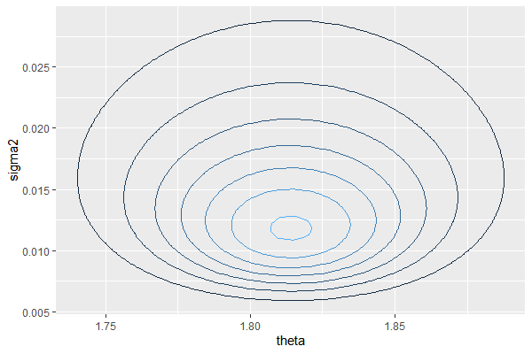
Then we can plot the posterior $p(\theta, \sigma^2|\mathbf{D})=p(\sigma^2|\mathbf{D})p(\theta|\sigma^2,\mathbf{D})$ as below.
# prior
mu0 = 1.9; kappa0 = 1
s20 = 0.01; nu0 = 1

# data
n = length(D)
xbar = mean(D)
s2 = var(D)

# posterior
kappa1 = kappa0 + n
nu1 = nu0 + n
mu1 = (kappa0 * mu0 + n * xbar) / kappa1
s21 = (1/ nu1) * (nu0*s20 + (n-1)*s2 + (kappa0*n/kappa1)*(xbar-mu0)^2 )

Theta = seq(1.6, 2.0, by = 0.005)
Sigma2 = seq(0, 0.04, by=0.0001)

library(invgamma)
posterior = function(theta, sigma2){
  dnorm(theta, mu1, sqrt(sigma2/kappa1)) * dinvgamma(sigma2, nu1/2, s21*nu1/2)
}

grid = outer(Theta, Sigma2, posterior)
rownames(grid) = Theta
colnames(grid) = Sigma2

df = melt(grid)
colnames(df) = c('theta','sigma2','density')

ggplot(df, aes(x=theta, y=sigma2, z=density))+
  geom_contour(aes(color=..level..))+
  guides(color=F)
Normal Model (Independent prior)
In some cases the dependence of $\theta$ on $\sigma^2$ might seem unreasonable. We consider independent prior $p(\theta, \sigma^2) =p(\theta)p(\sigma^2)$ as follows
$$
\begin{align}
\sigma^2 &\sim inv\Gamma(v_0/2, v_0\sigma^2_0/2)\\\
\theta &\sim N(\mu_0, \tau_0^2)
\end{align}
$$
In this case we can derive $p(\theta,\sigma^2|\mathbf{D})$ analytically, but we can compute
-
Joint Distribution of $\mathbf{D}, \sigma^2, \theta$
$$ p(\theta, \sigma^2, \mathbf{D})=p(\theta)p(\sigma^2)p(\mathbf{D}|\theta, \sigma^2) $$
-
Full conditional posterior of $\theta, \sigma^2$, in which case the prior is “semi” conjugate - prior and posterior is conjugate for one parameter only if all the other parameters are known.
$$
\begin{align}
p(\theta|\sigma^2, \mathbf{D}) &= dnorm(\theta, \mu_n, \tau_n^2)\\\
p(\sigma^2|\theta, \mathbf{D}) &= dinv\Gamma(\sigma^2, v_n, \dfrac{1}{v_n}[v_0\sigma_0^2+\sum (y_i-\theta)^2])
\end{align}
$$
We can numerically approximate $p(\theta,\sigma^2|\mathbf{D})$ by 1) compute $p(\theta, \sigma^2, \mathbf{D})$ for each possible pair of $(\theta, \sigma^2)$ (Grid Approximation) or sequentially generate sample pairs by using the full conditional posterior given above (Gibbs Sampler). Since grid approxmiation is nearly computationally infeasible in higher dimensions, so we consider Gibbs Sampler method, without justifying its usage just yet.
For any given pair ${\theta_s, \sigma^2_s}$, we generate the next sample ${\theta_{s+1}, \sigma^2_{s+1}}$ as
- sample $\theta_{s+1} \sim p(\theta|\sigma^2_s, \mathbf{D})$
- sample $\sigma^2_{s+1} \sim p(\sigma^2|\theta_{s+1}, \mathbf{D})$
For any initial pair (usually sample estimates) ${\theta_0, \sigma^2_0}$, it can be shown that a sequence of pairs generated from this iterative steps follows the joint posterior distribution $p(\theta, \sigma^2|\mathbf{D})$.
# prior
mu0 = 1.9; t20 = 0.95^2
s20 = 0.1; nu0 = 1

# data
n = length(D)
xbar = mean(D)
s2 = var(D)

# Gibbs sampler for posterior approximation
S = 1000
PHI = matrix(nrow = S, ncol = 2)
PHI[1,] = phi = c(xbar, s2) # sample estimate for initial value

set.seed(101)
for(s in 2:S){
  # sample theta (phi[2] = \sigma^2)
  mu1 = (mu0/t20 + n * xbar/ phi[2]) / (1/t20 + n / phi[2])
  t21 = 1/ (1/t20 + n/phi[2])
  phi[1] = rnorm(1, mu1, sqrt(t21))

  # sample sigma (phi[1] = \theta)
  nu1 = nu0 + n
  s21 = (nu0*s20 + (n-1)*s2 + n*(xbar - phi[1])^2)/nu1
  phi[2] = 1/rgamma(1, nu1/2, s21*nu1/2)

  PHI[s, ] = phi
}

PHI[,2] = sqrt(PHI[,2])
PHI_df = data.frame(PHI)
colnames(PHI_df) = c('theta','sigma')
ggplot(PHI_df, aes(x=theta, y=sigma))+
  geom_point()
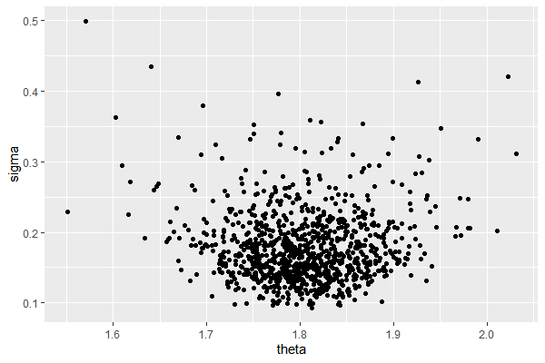
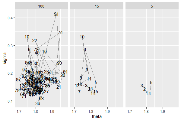
What happened under the hood is
PHI_df$n = 1:nrow(PHI_df)

one = head(PHI_df, n=5)
one$steps = '5'

two = head(PHI_df, n=15)
two$steps = '15'

thr = head(PHI_df, n=100)
thr$steps = '100'

phase = rbind(one, two, thr)
phase$steps = factor(phase$steps, levels=c('5','15','100'))
ggplot(phase, aes(x= theta, y= sigma))+
  geom_text(aes(label=n))+
  geom_path(alpha=0.4)+
  facet_wrap(~steps)
Remark: Is normal sampling assumption appropriate?
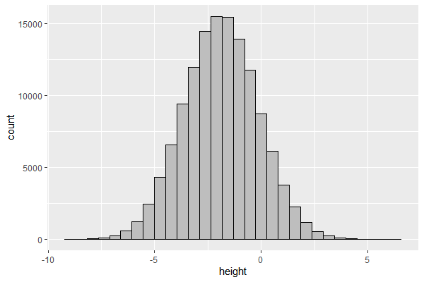
Apparently yes, if we assume that the data $x_i$ is an outcome of a large number of factors $\in {0,1}$ with additive effects $\beta_i$. For example,
$$ height = \beta_0 + \beta_1 gender + \beta_2 parent;tall + \beta_3 malnourished+… $$ With a simple simulation, we can see bell-shaped curve distribution for the height.
d = 50 # number of factors (variables)
N = 2^17 # number of observation
p = runif(d) # different distribution for each factor

factor = function(p){return(rbinom(N, 1, p))}
output = sapply(p, factor) # generate distribution of factors
beta = runif(d)*2-1 # generate beta for each factor

df = data.frame(height = output %*% beta)

ggplot(df, aes(x=height)) + geom_histogram(color='black',fill='grey', bins=30)
References
- First Course into Bayesian Statistical Analysis (Hoff, 2009)
- https://github.com/jayelm/hoff-bayesian-statistics