library(ggplot2)
library(cowplot)
library(reshape)

Multivariate Normal Model

Consider a bivariate normal random variable $[y_1, y_2]^T$. The density is written as ($p=2$)

$$ p(\mathbf{y}|\theta, \Sigma) = (\dfrac{1}{2\pi})^{-p/2}|\Sigma|^{-1/2} \exp{-\dfrac{1}{2}(\mathbf{y}-\theta)^T\Sigma^{-1}(\mathbf{y}-\theta)} $$

where the parameter is $\theta = \begin{pmatrix} E[y_1]\\\ E[y_2] \end{pmatrix}$ and $\Sigma = \begin{pmatrix} E[y_1^2]-E[y_1]^2 & E[y_1y_2]-E[y_1]E[y_2]\\\
E[y_2y_1]-E[y_2]E[y_1] & E[y_2^2]-E[y_2]^2 \end{pmatrix}$ $=\begin{pmatrix} \sigma_1^2 & \sigma_{12}\\\
\sigma_{21} & \sigma_2^1 \end{pmatrix}$.

Few things worth mentioning for multivariate normal model

1. the term in the exponent $(\mathbf{y}-\theta)^T\Sigma^{-1}(\mathbf{y}-\theta)$ is somewhat a measure of distance between mean and the data. Refer to https://en.wikipedia.org/wiki/Mahalanobis_distance

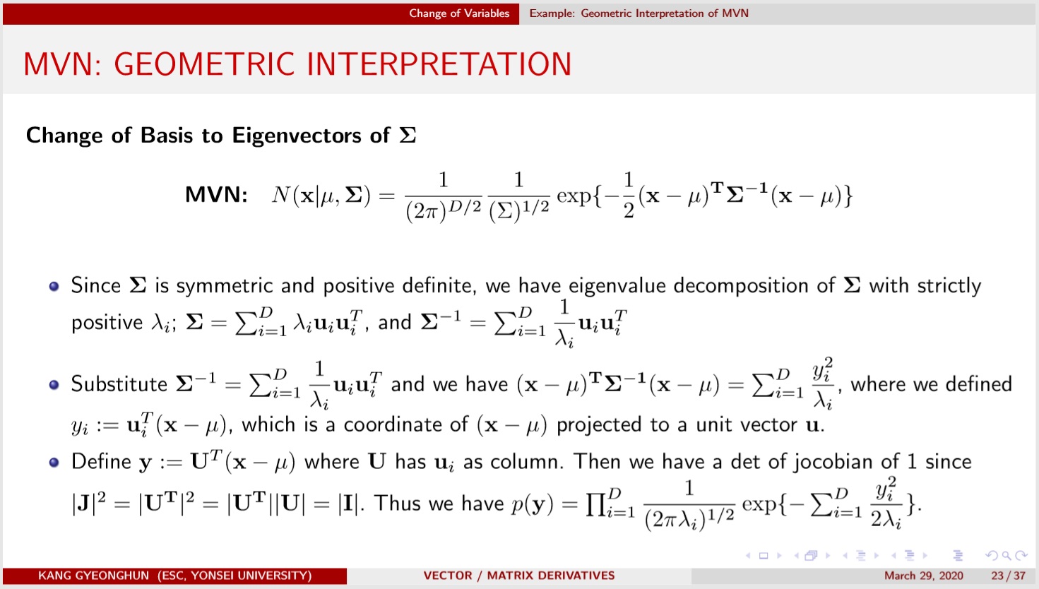
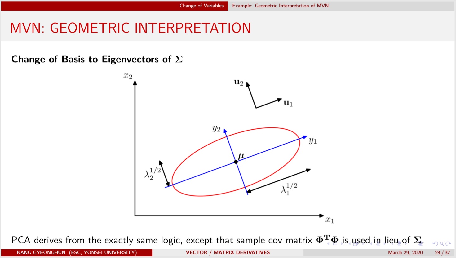
2. Geometrically, MVN density is spread along the eigenvectors of $\Sigma$, a symmetric postive definite matrix, with width determined by the corresponding eigenvalues. Refer to https://youtu.be/qvNhgkbzKmY?t=358

   

3. A bit of algebra shows that the MVN density can be written as

   $p(\mathbf{y}|\theta, \Sigma) = (\dfrac{1}{2\pi})^{-p/2}|\Sigma|^{-1/2} \exp(-\dfrac{1}{2}(\mathbf{y}-\theta)^T\Sigma^{-1}(\mathbf{y}-\theta))$ $\propto \exp(-\dfrac{1}{2}\mathbf{y}^T \Sigma^{-1}\mathbf{y} + \mathbf{y}^T\Sigma^{-1}\theta -\dfrac{1}{2}\theta^T \Sigma^{-1}\theta )$ $\propto\exp(-\dfrac{1}{2}\mathbf{y}^T \mathbf{A}\mathbf{y} +\mathbf{y}^T\mathbf{b})$ $(\theta = \mathbf{A^{-1}b},\quad \Sigma = \mathbf{A^{-1}})$

   This is useful in doing a multivariate version of “matching the exponents”.

Semiconjugate prior for the mean

For $\mathbf{D} = {\mathbf{y_1}, \mathbf{y_2}, …, \mathbf{y_n}}$ with $p$ variables, the joint likelihood density is

$$ p(\mathbf{D}|\theta, \Sigma) = (\dfrac{1}{2\pi})^{-np/2}|\Sigma|^{-n/2} \exp{-\dfrac{1}{2}\sum_{i=1}^n(\mathbf{y_i}-\theta)^T\Sigma^{-1}(\mathbf{y_i}-\theta)} $$

It seems natural to consider MVN as a prior for $\theta$ of MVN likelihood.

$$ \theta \sim MVN(\mu_0, \Lambda_0) $$

Then by (6), we see that

$$ \begin{align} p(\theta) &\propto \exp{ -\dfrac{1}{2}\theta^T\mathbf{A_0}\theta + \theta^T\mathbf{b_0}}\\\
\text{where}\quad & \mathbf{A_0} = \Lambda_0^{-1},\quad \mathbf{b_0}=\Lambda_0^{-1}\mu_0\\\
p(\mathbf{D}|\theta, \Sigma) &\propto \exp{ -\dfrac{1}{2}\theta^T\mathbf{A_1}\theta + \theta^T\mathbf{b_1}}\\\
\text{where}\quad & \mathbf{A_1} = n\Sigma^{-1},\quad \mathbf{b_1}=n\Sigma^{-1}\mathbf{\bar{y}}\\\
\therefore p(\theta|\mathbf{D},\Sigma) &\propto \exp{ -\dfrac{1}{2}\theta^T(\mathbf{A_0}+\mathbf{A_1})\theta + \theta^T(\mathbf{b_0}+\mathbf{b_1})}\\\
\end{align} $$

Hence the posterior for $\theta$ given $\mathbf{D}, \Sigma$ is

$$ \begin{align} \theta|\mathbf{D},\Sigma &\sim MVN(\mu_n, \Lambda_n)\\\
\mu_n &= (\Lambda_0^{-1}+n\Sigma^{-1})^{-1}(\Lambda_0^{-1}\mu_0+n\Sigma^{-1}\mathbf{\bar{y}})\\\
\Lambda_n &= (\Lambda_0^{-1}+n\Sigma^{-1})^{-1} \end{align} $$

which is reminiscent of the univariate normal case.

The inverse Wishart distribution for $\Sigma$ prior

When $y_i \sim N(\theta, \sigma^2)$, the sample variance follows chi-square (gamma) distribution. More generally, since $\frac{(n-1)s^2}{\sigma^2}\sim \Gamma(\frac{n-1}{2}, 2)$ we can write

$$ {(n-1)s^2} \sim \Gamma(\dfrac{n-1}{2}, \dfrac{1}{2\sigma^2}) $$

In univariate normal, the formula $(n-1)s^2=\sum_{i=1}^n (y_i - \bar{y})^2$ is called “the sum of squares”. We can come up with a similar formula for multivariate case as follows.

$$ \sum_{i=1}^n \mathbf{y_i}\mathbf{y_i^T} = \mathbf{Y^TY} \quad (\mathbf{Y}\in\mathbb{R}^{n\times p}) $$

If $\mathbf{y_i} \sim MVN(\mathbf{0}, \Phi_0)$, then $\mathbf{Y^TY}$ follows a Wishart distribution with parameters $(n, \Phi_0)$, which is analogous to the univariate case.

$\mathbf{Y^TY}$ is symmetric obviously, and also postive definite (as long as $n>p$) with probability 1. Using this result, we can construct an inverse Wishart prior for $\Sigma$ that is semi-conjugate.

Inverse Wishart Distribution

1. sample $\mathbf{y_i}\sim MVN(\mathbf{0}, \mathbf{S_0^{-1}})$
2. Calculate $\sum_{i=1}^{v_0} \mathbf{y_i}\mathbf{y_i^T} = \mathbf{Y^TY}$
3. set $\Sigma = \mathbf{Y^TY}^{-1}$.
4. $\Sigma \sim invW(v_0, \mathbf{S_0^{-1}})$, with $E[\Sigma]=\dfrac{\mathbf{S_0}}{v_0-p-1}$

Let $\Sigma_0$ be our prior guess on the true covariance matrix. Then we set $\mathbf{S_0}=(v_0+p+1)\Sigma_0$, and express our certainty with $v_0$. $v_0=p+2$ is only loosely centered on $\Sigma_0$.

It can be shown that the posterior is $\Sigma|\mathbf{D}, \theta \sim invW(v_0+n, (\mathbf{S_0}+\mathbf{S_\theta})^{-1})$ where $S_\theta = \sum_{i=1}^n(\mathbf{y_i}-\theta)(\mathbf{y_i}-\theta)^T$. The mean of the posterior is wegithed average of prior mean and sample covariance matrix, which is also comparable to single variable case.

$$ E[\Sigma|\mathbf{D}, \theta] = \dfrac{v_0-p-1}{v_0-p-1+n}\dfrac{\mathbf{S_0}}{v_0-p-1} +\dfrac{n}{v_0-p-1+n}\dfrac{\mathbf{S_\theta}}{n} $$

In summary, for MVN model, we have full conditional posteriors as follows, and we can use Gibbs Sampler to approximate the posterior.

Bayesian Linear Regression (fixed variance)

In linear regression with gaussian normal assumption we can write the likelihood of $\mathbf{y}$ as MVN with a mean which is a linear combination of coloumns of $\mathbf{X}$.

$$ \begin{align} \mathbf{y}|\mathbf{X}, \beta, \sigma^2 &\sim MVN(\mathbf{X\beta}, \sigma^2\mathbf{I})\\\
p(\mathbf{y}|\mathbf{X}, \beta, \sigma^2) &\propto \exp (-\dfrac{1}{2}\mathbf{(y-X\beta)^T(y-X\beta)}) \end{align} $$

With MVN prior on $\beta \sim MVN(\mathbf{\beta_0}, \Sigma_0)$, we see that

$$ \begin{align} p(\beta|\mathbf{y}, \mathbf{X}, \sigma^2) &\propto p(\mathbf{y}|\mathbf{X}, \beta, \sigma^2)p(\beta)\\\
&\propto \exp(-\dfrac{1}{2}\mathbf{(y-X\beta)^T(y-X\beta)}) \exp( -\dfrac{1}{2} \mathbf{(\beta-\beta_0)^T\Sigma_0^{-1}(\beta-\beta_0)} )\\\
&=\exp ( -\dfrac{1}{2}\beta^T(\Sigma_0^{-1}+\mathbf{X^TX}/\sigma^2)\beta+\beta^T(\Sigma_0^{-1}\beta_0 + \mathbf{X^Ty}/\sigma^2)) \end{align} $$

Again by (6), we see that the posterior for $\beta$ is also normal with

$$ \begin{align} V[\beta|\mathbf{y}, \mathbf{X}, \sigma^2] &= (\Sigma_0^{-1}+\mathbf{X^TX}/\sigma^2)^{-1}\\\
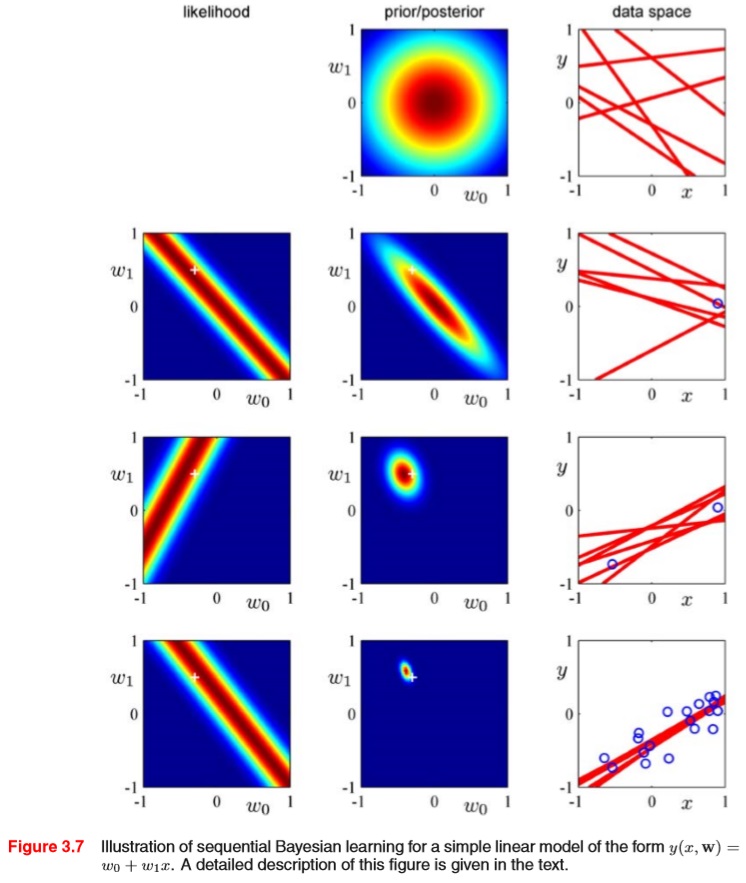
E[\beta|\mathbf{y}, \mathbf{X}, \sigma^2] &= (\Sigma_0^{-1}+\mathbf{X^TX}/\sigma^2)^{-1} (\Sigma_0^{-1}\beta_0 + \mathbf{X^Ty}/\sigma^2) \end{align} $$ The book PRML provides a great visualization of Bayesian linear regression. In the plot below, we have likelihood and prior/posterior drawn in a parameter space, and the set of parameters (slope and coefficient) is represented in the data space as a straight line. As more and more data are observed, from the corresponding likelihood for each newly arriving data, we get a posterior update which makes the belief more peaked at certain region, and this centralizing behavior is reflected as more and more coherent straight lines drawn in the data space.

Multinomial Model for categorical data

We can model a data with $k$ possible states as a multinomial model, and give a conjugate Dirichlet prior for the parameter $\theta_j$. Bayesian inference for this model is fairly simple, as the posterior is also Dirichlet with $\alpha_j$ added by the data count $y_j$. The example provides some details.

$$ \begin{align} \text{Likelihood}&\quad p(\mathbf{y}|\theta) \propto \prod_{j=1}^k \theta_j^{y_j} \quad (\mathbf{y}=[y_1, y_2, …, y_k]^T)\\\
\text{Prior}&\quad p(\theta) \propto \prod_{j=1}^k \theta_j^{\alpha_j-1} \quad (\text{parameters } \alpha_1, \alpha_2, …, \alpha_k)\\\
\text{Posterior}&\quad p(\theta|\mathbf{y}) \propto \prod_{j=1}^k \theta_j^{\alpha_j+y_j-1} \end{align} $$

Example: pre-election polling

library(DirichletReg)
# prior
a1 = a2 = a3 = 1 # weak prior

# data
y = c(727, 583, 137)

# posterior 
a1 = a1 + y[1]
a2 = a2 + y[2]
a3 = a3 + y[3]

# generate samples
set.seed(101)
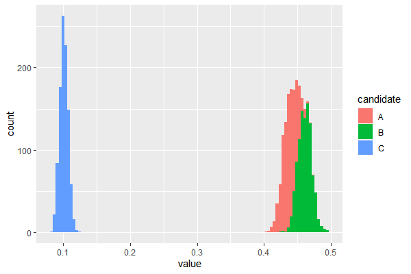
df = rdirichlet(1000, c(a1, a2, a3))
df = data.frame(df)
colnames(df) = c('A','B','C')

df_long = melt(df, variable_name = 'candidate')
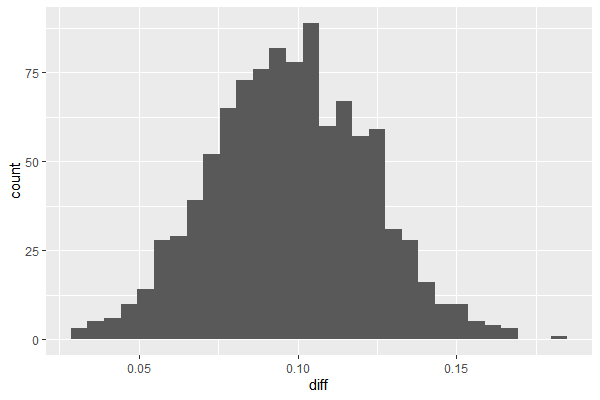
df_diff = data.frame(diff=df$A-df$B)

ggplot(df_long, aes(x=value, fill=candidate))+ geom_histogram(bins=100)
ggplot(df_diff, aes(x=diff)) + geom_histogram(bins=30)

# new data
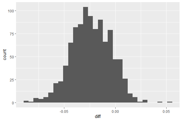
y = c(300, 500, 100)
a1 = a1 + y[1]
a2 = a2 + y[2]
a3 = a3 + y[3]

# generate samples
df = rdirichlet(1000, c(a1, a2, a3))
df = data.frame(df)
colnames(df) = c('A','B','C')

df_long = melt(df, variable_name = 'candidate')
df_diff = data.frame(diff=df$A-df$B)

ggplot(df_long, aes(x=value, fill=candidate))+geom_histogram(bins=100)
ggplot(df_diff, aes(x=diff)) + geom_histogram(bins=30)

References

1. First Course into Bayesian Statistical Methods (Hoff, 2009)
2. https://github.com/jayelm/hoff-bayesian-statistics
3. Pattern Recognition and Machine Learning (Bishop, 2006) (figures)