
Mixtures of Gaussians and EM algorithm
When the typical Maximum-Likelihood approach leads you astray
Mixtures of Gaussians (GMM)
GMM as a joint distribution
Suppose a random vector $\mathbf{x}$ follows a $K$ Gaussian mixture distribution,
$$ p(\mathbf{x}) = \sum_{k=1}^K \pi_k N(\mathbf{x}\mid \boldsymbol{\mu_k, \Sigma_k}) $$
Knowing the distribution means we have complete information about the set of parameters $\pi_k, \boldsymbol{\mu_k, \Sigma_k}$ for all $k$. Let us say that the parameter $\pi_k$ is shrouded, and instead we have a random variable $\mathbf{z}$ with $1-to-K$ coding where exactly one of $K$ elements (say $z_k$) be $1$ while all else are $0$. Say it follows a multinomial distribution with $\pi_k$ under the constraint $\sum_{k}\pi_k=1$. Then its density can be written as
$$
\begin{align}
\text{Latent variable}\quad \mathbf{z}&=[z_1, …,z_K] \sim multinomial(\pi_k)\\\
p(\mathbf{z})&= \prod_{k=1}^K \pi_k^{z_k}
\end{align}
$$
Similarly, given that $z=k$, we can think of $N(\mathbf{x}\mid \boldsymbol{\mu_k, \Sigma_k})$ as $p(\mathbf{x} \mid z_k=1)$. Then we have another formulation of $K$ Gaussian mixture as
$$
\begin{align}
p(\mathbf{x,z})&= p(\mathbf{z})p(\mathbf{x\mid z}) = \prod_{k=1}^K\pi_k^{z_k}N(\mathbf{x}\mid \boldsymbol{\mu_k, \Sigma_k})^{z_k}=\pi_kN(\mathbf{x}\mid \boldsymbol{\mu_k, \Sigma_k})\\\
p(\mathbf{x})&= \sum_{z}p(\mathbf{x,z})=\sum_{k=1}^K\pi_kN(\mathbf{x}\mid \boldsymbol{\mu_k, \Sigma_k})
\end{align}
$$
Does not seem to have changed at all, but we in fact introduced a latent variable $z$, and the above formula makes it explicit the fact that $p(\mathbf{x})$ is actually a marginal of the joint distribution; $p(\mathbf{x})=\sum_z p(\mathbf{z,x})$. With the joint $p(\mathbf{z,x})$, we can go further to discuss $\gamma(z_k)=p(z_k=1\mid \mathbf{x})$, which can be obtained with Bayes rule;
$$ \begin{align} p(\mathbf{z\mid x})=p(z_k=1\mid \mathbf{x})&= \dfrac{p(k)p(\mathbf{x}\mid k)}{\sum_j^Kp(j)p(\mathbf{x}\mid j)}=\dfrac{\pi_k N(\mathbf{x}\mid \boldsymbol{\mu_k, \Sigma_k})}{\sum_j^K\pi_j N(\mathbf{x}\mid \boldsymbol{\mu_j, \Sigma_j})}=\gamma(z_k) \end{align} $$
Note that $z$ indicates an assignment of the data vector $\mathbf{x}$ to one of $1,2,…,K$ Gaussians. In a sense, $\pi_k$ is the probability that $\mathbf{x}$ is in $k$th Gaussian regardless of (prior to) the data $\mathbf{x}$, and $\gamma(z_k)=p(z_k=1\mid \mathbf{x})$ is the probability that $\mathbf{x}$ is in $k$th Gaussian after observing the value $\mathbf{x}$.
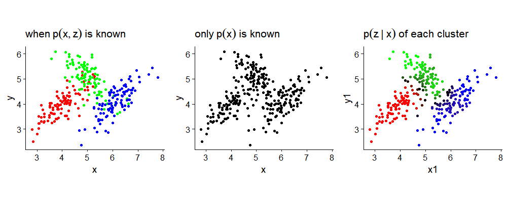
The following plots illustrate the difference between $p(\mathbf{z,x})$, $p(\mathbf{z}\mid \mathbf{x})$ and $p(\mathbf{x})$. Complete knowledge of the distribution $p(\mathbf{z,x})$ means that not only $\boldsymbol{\mu_k, \Sigma_k}$ bus also $\pi_k$ is also given, which enables us to color each dot correctly according to $k$th Gaussians. We can sample from $p(\mathbf{z,x})$ by first generating $z\sim multi(\pi_k)$, and then sampling from $N(\boldsymbol{\mu_k, \Sigma_k})$. Since we know $p(\mathbf{z,x})$, we can also plot as in the second graph $p(\mathbf{z}\mid \mathbf{x})$ for each data by using (7). Lastly, without any knowledge of all the parameters, we have $p(\mathbf{x})$.
Inference on GMM: ill-posed MLE problem
For $N\times D$ data set $\mathbf{X}$ where each row is an observation $\mathbf{x_n^T}$, we introduce a latent variable $z_{nk}\sim multinomial(\pi_k)$ which indicates an assignment of data $\mathbf{x_n}$ to $k$th Gaussian. The likelihood for the entire data set is
$$ \begin{align} p(\mathbf{X}\mid \boldsymbol{\pi, \mu, \Sigma})=\prod_{n=1}^N\Bigg(\sum_{k=1}^K \pi_k N(\mathbf{x_n}\mid \boldsymbol{\mu_k, \Sigma_k})\Bigg) \end{align} $$
where $\boldsymbol{\pi, \mu, \Sigma}$ is a complete set of parameters to specify Mixtures of Gaussians. Taking a log, we have
$$ \begin{align} \ln p(\mathbf{X}\mid \boldsymbol{\pi, \mu, \Sigma})=\sum_{n=1}^N\ln\Bigg(\sum_{k=1}^K \pi_k N(\mathbf{x_n}\mid \boldsymbol{\mu_k, \Sigma_k})\Bigg) \end{align} $$
Our goal is to find $\boldsymbol{\pi, \mu, \Sigma}$ that maximize this likelihood, but there are several problems associated with MLE framework in GMM. Unlike in a single Gaussian case, the likelihood for GMM can go to infinity, so the maximum likelihood framework is not necessarily appropriate approach. To see why, consider the following example.
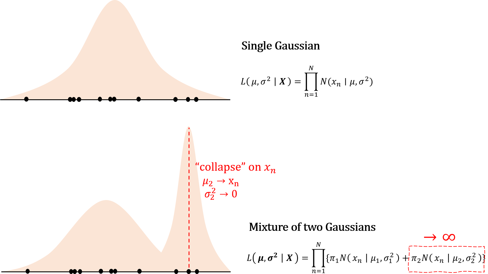
For a single Gaussian, if the density falls on one single point, then the density at that particular region gets infinitely large, but this effect is countered by decreasing density in other data points as $\sigma^2 \to 0$. However, for a mixture of Gaussians, even as $\sigma^2_2 \to 0$, variance (width) of other Gaussians does not decrease accordingly.
Furthermore, since there is no ordering for $K$ set of parameters, there can be a total of $K!$ equivalent solutions for MLE, which makes the likelihood for GMM “unidentifiable”. This could be trivial as any of the $K!$ is as good as others for clustering purpose. Even so, taking a derivative of the log likelihood yields an unholy mass because unlike in a single Gaussian case, in GMM normal densities are all clumped together inside the logarithm.
Numerical solution: EM for GMM
For reasons detailed above, we cannot get a closed form solution for GMM. Instead, we can use three partial derivative conditions that MLE should satisfy. But since the solution is all implicit in its form, the algorithm must be iterative, and the convergence might not be either unique or globally optimal.
Suppose the assignment probability $\pi_k$ are all given. The MLE of the likelihood of GMM must suffice the following first derivative conditions
$$ \begin{align} \dfrac{\partial logL}{\partial \boldsymbol{\mu_k}} = -\sum_{n=1}^N\dfrac{\pi_k N(\mathbf{x_n}\mid \boldsymbol{\mu_k, \Sigma_k})}{\sum_j^K\pi_j N(\mathbf{x_n}\mid \boldsymbol{\mu_j, \Sigma_j})} \boldsymbol{\Sigma_k}(\mathbf{x_n}-\boldsymbol{\mu_k})=0, \quad \dfrac{\partial logL}{\partial \boldsymbol{\Sigma_k}} =0 \end{align} $$
which leads to a solution
$$
\begin{align}
\boldsymbol{\mu_k} &= \dfrac{1}{N_k}\sum_{n=1}^N \gamma(z_{nk})\mathbf{x_n}\\\
\boldsymbol{\Sigma_k} &= \dfrac{1}{N_k}\sum_{n=1}^N\gamma(z_{nk})(\mathbf{x_n}-\boldsymbol{\mu_k})(\mathbf{x_n}-\boldsymbol{\mu_k})^T
\end{align}
$$
where we defined $\gamma(z_{nk})=\frac{\pi_k N(\mathbf{x_n}\mid \boldsymbol{\mu_k, \Sigma_k})}{\sum_j^K\pi_j N(\mathbf{x_n}\mid \boldsymbol{\mu_j, \Sigma_j})}$ and $N_k=\sum_{n=1}^N \gamma(z_{nk})$. Note that the above solution is almost identical to MLE for a single multivariate normal density, except that we get a weighted average for sample mean and covariance for each $k$. For each data vector, $\gamma(z_{nk})=p(z_{nk}\mid \mathbf{x_n})$ is a probability that $\mathbf{x_n}$ belongs to $k$th Gaussian, so for each data vector we have a cluster-assignment distribution. In this sense, the sum of $\gamma(z_{nk})$ for $k$th class can be interpreted as an effective number of observations in $k$th class. Since $\gamma(z_{nk})$ also contains $\boldsymbol{\mu_k, \Sigma_k}$, the above solution is implicit, not in a closed form.
Next, for a given $\boldsymbol{\mu_k, \Sigma_k}$, obtaining the MLE solution of $\pi_k$ is to solve a Lagrange multiplier problem where the objective function to maximize is the likelihood function and the equality constraint is $\sum_{k=1}^K \pi_k=1$.
$$
L = \sum_{n=1}^N\log p(\mathbf{x_n}\mid \boldsymbol{\pi, \mu, \Sigma})+\lambda \Big( \sum_{k=1}^K\pi_k-1\Big)\\\
\dfrac{\partial L}{\partial \pi_k} = \sum_{n=1}^N\dfrac{N(\mathbf{x_n}\mid \boldsymbol{\mu_k, \Sigma_k})}{\sum_j \pi_j N(\mathbf{x_n}\mid \boldsymbol{\mu_j, \Sigma_j})}+\lambda =^{let}0
$$
This yields a solution
$$ \pi_k = \dfrac{\sum_{n=1}^N \frac{\pi_k N(\mathbf{x_n}\mid \boldsymbol{\mu_k, \Sigma_k})}{\sum_j^K\pi_j N(\mathbf{x_n}\mid \boldsymbol{\mu_j, \Sigma_j})}}{N} = \dfrac{N_k}{N} $$
which is also in an implicit form. Now we have an iterative algorithm:
EM Algorithm for GMM
- Initialize $\boldsymbol{\mu_k, \Sigma_k, \pi_k}$ (usually by K-means for computational convenience)
- E-step: update the cluster-assignment distribution $\gamma(z_{nk})$
- M-step: update $\boldsymbol{\mu_k, \Sigma_k, \pi_k}$
- Evaluate the log likelihood and check for convergence. If not, repeat 2~4.
To recap, in GMM, our objective is to maximize the likelihood function w.r.t. $\boldsymbol{\pi, \mu, \Sigma}$, ($\mathbf{X}$: $N\times D$ matrix)
$$
\begin{align*}
\arg\max p(\mathbf{X} \mid \boldsymbol{\pi, \mu, \Sigma})=\prod_{n=1}^N\Big(\sum_{k=1}^K \pi_k N(\mathbf{x_n}\mid \boldsymbol{\mu_k, \Sigma_k})\Big)\\\
\arg\max \log p(\mathbf{X} \mid \boldsymbol{\pi, \mu, \Sigma})=\sum_{n=1}^N\ln\Big(\sum_{k=1}^K \pi_k N(\mathbf{x_n}\mid \boldsymbol{\mu_k, \Sigma_k})\Big)
\end{align*}
$$
But this likelihood is intractable. Suppose instead that we are given a $N \times K$ matrix of hidden variables $\mathbf{Z}$ where $z_{nk}=1$ indicates $\mathbf{x_n}$ belongs to $k$th Gaussian. That is, we have a complete data $\mathbf{X,Z}$. Then finding MLE of the joint distribution is fairly straightforward for GMM.
$$
\begin{align}
\arg\max p(\mathbf{X}, \mathbf{Z} \mid \boldsymbol{\pi, \mu, \Sigma}) &= \prod_{n=1}^N \prod_{k=1}^K
\pi_k^{z_{nk}}N(\mathbf{x_n}\mid \boldsymbol{\mu_k,\Sigma_k})^{z_{nk}}\\\
\arg\max \log p(\mathbf{X}, \mathbf{Z} \mid \boldsymbol{\pi, \mu, \Sigma}) &= \sum_n \sum_k z_{nk}(\log \pi_k + \log N(\mathbf{x_n}\mid \boldsymbol{\mu_k,\Sigma_k}))
\end{align}
$$
Unlike $\log p(\mathbf{X} \mid \boldsymbol{\pi, \mu, \Sigma})$, every term in $\log p(\mathbf{X}, \mathbf{Z} \mid \boldsymbol{\pi, \mu, \Sigma})$ has been separated after log transformation. In fact, with $\mathbf{Z}$, we have a classification problem where class conditional density is multivariate normal, which is an assumption of QDA. Thus MLE for $\boldsymbol{\pi, \mu, \Sigma}$ is equal to that of QDA; sample proportion of class $k$, sample mean and covariance of data vectors in class $k$ respectively.
The only problem is that we do not have the label $z_{nk}$ in GMM clustering problem, so we cannot calculate the complete data log likelihood $\log p(\mathbf{X}, \mathbf{Z} \mid \boldsymbol{\pi, \mu, \Sigma})$. Instead, in the EM algorithm suggested above we have calculated
$$ \begin{align} J=\sum_n \sum_k &\gamma(z_{nk})(\log \pi_k + \log N(\mathbf{x_n}\mid \boldsymbol{\mu_k,\Sigma_k})) \end{align} $$
In fact, this is an expectation of the complete data log likelihood, provided that $z_{nk}$ follows the distribution $z_{nk}\sim p(z_{nk}=1 \mid \mathbf{x_n})= \gamma(z_{nk})$.
$$ J=E_{\mathbf{Z\mid X}}[\log p(\mathbf{X}, \mathbf{Z} \mid \boldsymbol{\pi, \mu, \Sigma})] $$
Given an initial value $\boldsymbol{\mu_k, \Sigma_k, \pi_k}$, the algorithm calculates $\gamma(z_{nk})$ which is to get an expectation value $J$ (E-step), and maximizes it by updating $\boldsymbol{\mu_k, \Sigma_k, \pi_k}$ (M-step), and after enough iterations $J$ converges to some desired local maximum. How so? That would be a topic of the next post!
EM for Gaussian Mixtures in R
hun_EM = function(df, K, tol=0.01){

  df = data.matrix(df)
  n = nrow(df)
  d = ncol(df)

  # 0. initialize pr, mu, sigma
  km = hun_kmeans(df, K)
  pr = matrix(rep(1/K, K), ncol=K)
  mu = array(t(km$mu), dim=c(2,1,2))
  sigma = array(rep(diag(d),K), dim=c(d,d,K))


  # 0. calculate log likelihood

  dmnorm = function(y, Theta, Sigma){
    y = as.matrix(y)
    Theta = as.matrix(Theta)
    Sigma = as.matrix(Sigma)
    p = nrow(Theta)
    (2*pi)^(-p/2)*det(Sigma)^(-1/2)*
      exp(-t(y-Theta) %*% solve(Sigma) %*% (y - Theta) /2)
  }

  prob_per_k = function(x, pr, mu, sigma){
    lik = rep(0, K)
    for(k in 1:K){
      lik[k] = dmnorm(x, mu[,,k], sigma[,,k])*pr[k]
    }
    lik # output 1xK vector of pr*N(x|mu, sigma)
  }

  z = t(apply(df, 1, function(x) prob_per_k(x, pr, mu, sigma)))
  loglik = sum(log(rowSums(z)))

  convergence = F
  count = 0
  # 1. do EM until convergence

  while(convergence==F){
    # E: update responsibility (cond exp of hidde variable z)
    z = t(apply(z, 1, function(x) x/sum(x)))

    # M: update parameters
    pr = colSums(z)/n
    for(k in 1:K){
      mu[,,k] = colSums(df*z[,k]) /colSums(z)[k]
      Mu = matrix(rep(1, n), ncol=1) %*% mu[,,k]
      sigma[,,k] =  t(df-Mu) %*% ((df - Mu)* z[,k])/colSums(z)[k]
    }

    # check: calculate log likelihood
    z = t(apply(df, 1, function(x) prob_per_k(x, pr, mu, sigma)))
    loglik_new = sum(log(rowSums(z)))
    convergence = (abs(loglik_new-loglik) < tol)
    loglik = loglik_new
    count = count+1
  }

  output = list(mu=mu, sigma=sigma, pr=pr, loglik=loglik, count=count)
  return(output)
}
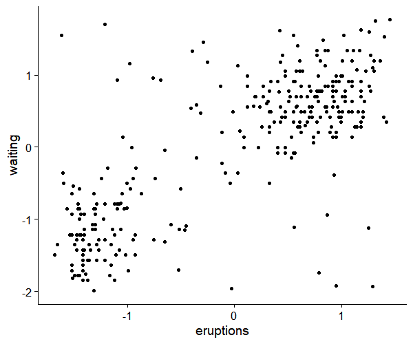
## faithful data ##
library(ggplot2)
library(cowplot)
library(reshape)

set.seed(101)
nNoise = 50
Noise = apply(faithful, 2, function(x)
  runif(nNoise, min=min(x)-0.1, max=max(x)+0.1))
df = rbind(faithful, Noise)
df = apply(df, 2, function(x){return((x-mean(x))/sd(x))})

ggplot(data.frame(df), aes(x=eruptions, y=waiting))+
  geom_point()+
  theme_cowplot()
## plot result ##
set.seed(101)
result = hun_EM(df, 2)
dmnorm = function(y, Theta, Sigma){
y = as.matrix(y)
Theta = as.matrix(Theta)
Sigma = as.matrix(Sigma)
p = nrow(Theta)
(2*pi)^(-p/2)*det(Sigma)^(-1/2)*
exp(-t(y-Theta) %*% solve(Sigma) %*% (y - Theta) /2)
}
dGMM = function(x, pr, mu, sigma){
K = length(pr)
lik = rep(0, K)
for(k in 1:K){
lik[k] = dmnorm(x, mu[,,k], sigma[,,k])*pr[k]
}
sum(lik)
}
y1 = seq(-2, 2, length=100)
y2 = seq(-2, 2, length=100)
calc.density = Vectorize(function(y1, y2){
y = c(y1, y2)
dGMM(y, result$pr, result$mu, result$sigma)
})
grid = outer(y1, y2, FUN = calc.density)
rownames(grid) = y1
colnames(grid) = y2
grid = melt(grid)
colnames(grid)= c('eruptions','waiting','density')
density = apply(df, 1, function(x) dGMM(x, result$pr, result$mu, result$sigma))
df = cbind(df, density)
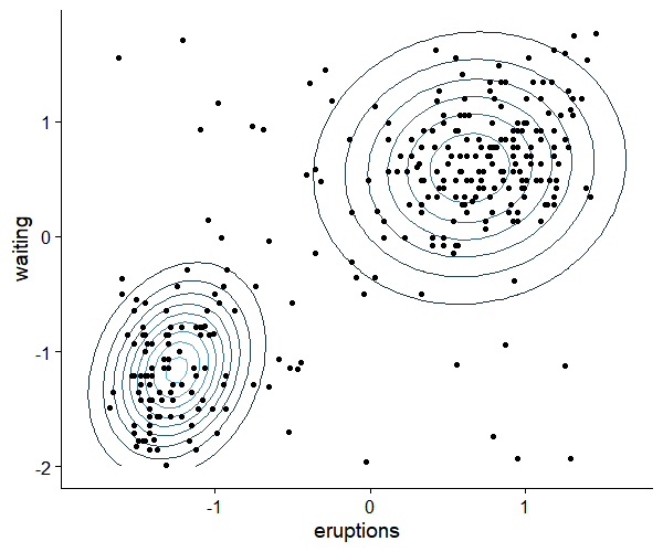
ggplot(grid, aes(x=eruptions, y=waiting, z=density))+
geom_contour(aes(color=..level..))+
geom_point(data=data.frame(df), aes(x=eruptions, y=waiting))+
guides(color=FALSE)+
theme_cowplot()
References
- Pattern Recognition and Machine Learning, Bishop, 2006
- https://bloomberg.github.io/foml/#lectures