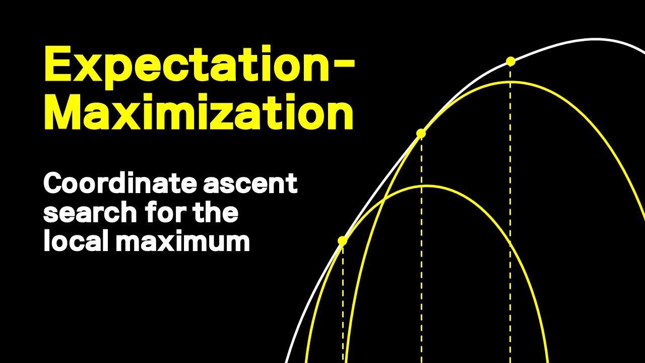
EM Algorithm for Latent Variable Models

For an observed data $\mathbf{x}$, we might posit the existence of an unobserved data $\mathbf{z}$ and include it in model $p(\mathbf{x,z}\mid \theta)$. This is called a latent variable model. The question is, why bother? It turns out that in many cases, learning $\theta$ with the marginal log likelihood $p(\mathbf{x}\mid \theta)$ is hard, whereas learning with the joint likelihood with a complete data set $p(\mathbf{x,z}\mid \theta)$ is relatively easy. GMM is one such case. With all the labels, fitting GMM relegates to fitting QDA with a nice and neat closed form solution. Even if $\mathbf{z}$ is unobserved, with an appropriate distribution for $\mathbf{z}$, can still obtain a reasonably satisfiable lower bound of $p(\mathbf{x}\mid \theta)$.

Suppose we want $\max_{\theta} \log p(\mathbf{x}\mid\theta)$. Let $q(\mathbf{z})$ be any distribution for the latent variable. Then we have

$$ \begin{align} \log p(\mathbf{x}\mid \theta) &= \log \Bigg[\sum_z p(\mathbf{x,z}\mid \theta)\Bigg] =\log \Bigg[\sum_z q(\mathbf{z})\dfrac{p(\mathbf{x,z}\mid \theta)}{q(\mathbf{z})}\Bigg]\\\
&=\log E_q\Bigg[ \dfrac{p(\mathbf{x,z}\mid \theta)}{q(\mathbf{z})}\Bigg]\\\
&\geq E_q\Bigg[\log \dfrac{p(\mathbf{x,z}\mid \theta)}{q(\mathbf{z})} \Bigg] = \sum_z q(\mathbf{z})\log\dfrac{p(\mathbf{x,z}\mid \theta)}{q(\mathbf{z})} := L(q, \theta) \quad \text{ELBO} \end{align} $$

That is, for any $q$ and $\theta$, we have ELBO, a lower bound for the evidence function $p(\mathbf{x}\mid \theta)$ (the name “evidence” comes from Bayesian context)

$$ \log p(\mathbf{x}\mid \theta)\geq \sum_z q(\mathbf{z})\log\dfrac{p(\mathbf{x,z}\mid \theta)}{q(\mathbf{z})} = L(q, \theta) $$

Then instead of one shot maximization of the marginal log likelihood ($\theta_{MLE}=\arg\max_{\theta}\log p(\mathbf{x}\mid \theta)$), we can maximize its lower bound $L(q,\theta)$ iteratively until it reaches some local maximum;

$$ \theta^t_{EM} = \arg\max_{\theta}\Big[ \max_{q} L(q, \theta) \Big]\quad \text{for t=1:n iterations} $$

Perhaps this plot from PRML might understand what is going on here. $L(q, \theta)$ is a lower bound for the red graph $\log p(\mathbf{x}\mid \theta)$.

• For any given $\theta^{old}$, find a distribution of a latent variable $q(\mathbf{z})$ so that $\sum_z q(\mathbf{z})\log\dfrac{p(\mathbf{x,z}\mid \theta)}{q(\mathbf{z})} = L(q, \theta)$ is maximized. When drawn with respect to $\theta$, this corresponds to the blue curve. Note that at $\theta^{old}$ the blue curve touches the red one.
• Along the blue curve (for a fixed $q$), find the value of $\theta^{new}$ with a maximum $L(q, \theta)$, which is the mode of the blue curve.
• Again, at $\theta^{new}$, jump to the green curve (update $q$).

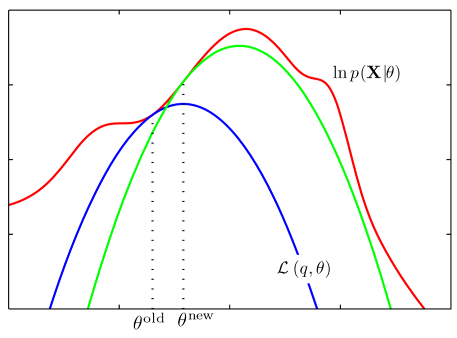
(source: PRML)

We can see that with this ‘coordinate ascent’, EM algorithm gives a sequence of $\theta$ that is monotonically increasing. To see why, note that $\log p(\mathbf{x}\mid \theta^{new}) \geq L(q, \theta^{new}) \geq L(q, \theta^{old} ) =\log p(\mathbf{x}\mid \theta^{old})$

How to update $q, \theta$?

How to update $q$ at a fixed $\theta$?

We can interpret ELBO in terms of KL divergence.

$$ \begin{align} L(q, \theta)&= \sum_z q(\mathbf{z})\log\dfrac{p(\mathbf{x,z}\mid \theta)}{q(\mathbf{z})}\\\
&= \sum_z q(\mathbf{z})\log\dfrac{p(\mathbf{z}\mid \mathbf{x}, \theta)p(\mathbf{x}\mid \theta)}{q(\mathbf{z})} \\\
&= \sum_z q(\mathbf{z})\log\dfrac{p(\mathbf{z}\mid \mathbf{x}, \theta)}{q(\mathbf{z})}+ \sum_z q(\mathbf{z})\log p(\mathbf{x}\mid\theta)\\\
&=-KL(q(\mathbf{z}) | p(\mathbf{z} \mid \mathbf{x},\theta))+\log p(\mathbf{x}\mid\theta) \end{align} $$

where the last line follows from $\sum_z q(z)\log p(x\mid \theta) = E_z(\log p(x\mid \theta))=\log p(x\mid \theta)$.

For a fixed $\theta$, the difference between the evidence $\log p(\mathbf{x}\mid \theta)$ and the ELBO $L(q, \theta)$ is KL divergence $KL(q(\mathbf{z}) | p(\mathbf{z} \mid \mathbf{x},\theta))$, so the choice of $q$ must be $p(\mathbf{z} \mid \mathbf{x},\theta)$ for a fixed parameter $\theta$. In other words, for any $\theta$, the choice of $p(\mathbf{z} \mid \mathbf{x},\theta)$ as $q$ guarantees that ELBO would be “touching” the evidence $\log p(\mathbf{x}\mid \theta)$, as we see in the figure above where the blue and the green curve touch the red one at $\theta^{old}$ and $\theta^{old}$ respectively.

How to update $\theta$ at a fixed $q$?

Again, we have

$$ \begin{align} L(q, \theta) &= \sum_z q(\mathbf{z})\log\dfrac{p(\mathbf{x,z}\mid \theta)}{q(\mathbf{z})}\\\
&= \sum_z q(\mathbf{z})\log p(\mathbf{x,z}\mid \theta) -\sum_z q(\mathbf{z})\log q(\mathbf{z}) \end{align} $$

So for a fixed $q$ maximizing $L(q, \theta)$ is to maximize the expectation of the complete log likelihood $E_q[\log p(\mathbf{x,z}\mid\theta)]$ given that $\mathbf{z} \sim q$.

In summary,

General EM Algorithm

1. Choose initial $\theta^{old}$
2. Expectation step:
   1. Let $q = p(\mathbf{z} \mid \mathbf{x}, \theta^{old})$
   2. Let $J(\theta):= L(q, \theta^{old}) = E_z[\log \dfrac{p(\mathbf{x,z}\mid \theta)}{q(\mathbf{z})}]$
3. Maximization step: let $\theta^{old} = \arg\max_{\theta}J(\theta)=\arg\max_{\theta} E_q[\log p(\mathbf{x,z}\mid\theta)]$
4. Repeat 2~3 until convergence

More Mathematical Details

1. We can say for certain that once we found the global maximum of $L(q, \theta)$ (if it exists, of course), then $\theta$ is a global maximum of $\log p(\mathbf{x}\mid\theta)$. For any other $\theta_t \not = \theta$, $\log p(\mathbf{x} \mid \theta_t) = L(q_t,\theta_t)+KL(q_t |p(\mathbf{z}\mid \mathbf{x}, \theta_t))=L(q_t,\theta_t)\leq L(q, \theta) = \log p(\mathbf{x} \mid \theta)$, where $q_t = p(\mathbf{z}\mid \mathbf{x}, \theta_t)$.
2. Under some regularity condition on the likelihood $p(\mathbf{x}\mid \theta)$, EM algorithm reaches some stationary point of $p(\mathbf{x}\mid \theta)$ which is a fixed point of EM.

References

1. Pattern Recognition and Machine Learning, Bishop, 2006
2. https://bloomberg.github.io/foml/#lectures