library(ggplot2) library(cowplot) library(reshape) Multivariate Normal Model Consider a bivariate normal random variable $[y_1, y_2]^T$. The density is written as ($p=2$)
$$ p(\mathbf{y}|\theta, \Sigma) = (\dfrac{1}{2\pi})^{-p/2}|\Sigma|^{-1/2} \exp{-\dfrac{1}{2}(\mathbf{y}-\theta)^T\Sigma^{-1}(\mathbf{y}-\theta)} $$
where the parameter is $\theta = \begin{pmatrix} E[y_1]\\\ E[y_2] \end{pmatrix}$ and $\Sigma = \begin{pmatrix} E[y_1^2]-E[y_1]^2 & E[y_1y_2]-E[y_1]E[y_2]\\\
E[y_2y_1]-E[y_2]E[y_1] & E[y_2^2]-E[y_2]^2 \end{pmatrix}$ $=\begin{pmatrix} \sigma_1^2 & \sigma_{12}\\\
\sigma_{21} & \sigma_2^1 \end{pmatrix}$.
Few things worth mentioning for multivariate normal model
the term in the exponent $(\mathbf{y}-\theta)^T\Sigma^{-1}(\mathbf{y}-\theta)$ is somewhat a measure of distance between mean and the data.
Inference for Normal Model Normal likelihood model has two parameters
$$ p(x|\theta, \sigma^2) = \dfrac{1}{\sigma\sqrt{2\pi}}\exp(-\dfrac{1}{2}(\dfrac{x-\theta}{\sigma})^2) $$ which requires a joint prior $p(\theta, \sigma^2)$. As for a single parameter case, we have joint posterior updated as
$$ p(\theta, \sigma^2|\mathbf{D}) \propto p(\theta, \sigma^2)p(\mathbf{D}|\theta, \sigma^2) $$ When our interest is in $\theta$, $\sigma^2$ is a nuisance parameter. Given the data $\mathbf{D}$ and the normal likelihood, we have three ways to deal with $\sigma^2$;
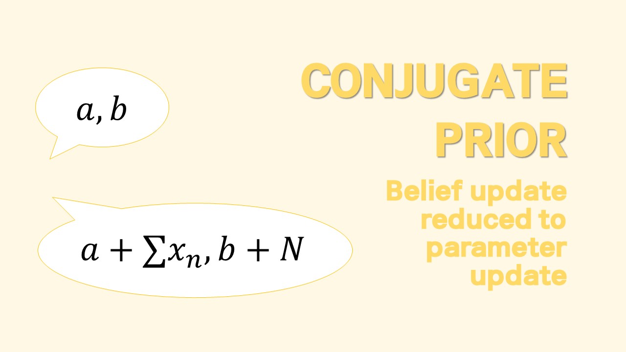
library(ggplot2) library(cowplot) library(reshape) Bayesian Update and Prediction Given a data $\mathbf{D}={x_1, x_2, …, x_n}$, once a likelihood model $p(\mathbf{D}|\theta)$ and a prior on a parameter $p(\theta)$ are specified, Bayesian inference produces an updated belief on $\theta$.
$$ \begin{align} \text{Prior Belief}&\quad p(\theta)\\\
\text{Likelihood}&\quad p(\mathbf{D}|\theta)\\\
\text{Updated (Posterior)}&\quad p(\theta|\mathbf{D}) = \dfrac{p(\mathbf{D}|\theta)p(\theta)}{\int p(\mathbf{D}|\theta)p(\theta)d\theta} \propto p(\mathbf{D}|\theta)p(\theta) \end{align} $$
Our interest may extend to the prediction the new value $\tilde{x}$ that would be generated from the same sampling distribution.